How Vegetation Indices Improve Maize Growth Monitoring

Maize is the world’s most produced cereal crop by volume, with the United States alone planting across approximately 35 million hectares and producing 390 million metric tons in 2023. Managing a crop at that scale demands more than scouting on foot. Vegetation indices for maize growth monitoring — mathematical formulas derived from the way plant canopies reflect and absorb light — have become a cornerstone of modern crop management because they translate spectral data into actionable crop health information. They do this fast, at scale, and without touching a single leaf.

Remote sensing technology, now available through satellites, drones, and handheld sensors, feeds real-time spectral data into these indices at every stage of the maize growing season. A farmer or agronomist can detect nitrogen stress at V6 before the leaves turn yellow, spot water deficit during grain fill before yields drop, or calibrate variable-rate fertilizer applications using canopy maps generated the same week the crop needs feeding.

What Are Vegetation Indices? How It Work?

A vegetation index (VI) is a dimensionless, quantitative value calculated by mathematically combining the reflectance values of two or more spectral bands captured by a sensor. The result is a single number that isolates and amplifies specific biological characteristics of a plant canopy — such as chlorophyll concentration, leaf area, or water content — while suppressing interference from soil, atmosphere, and shadow.

The power of a vegetation index lies in its ability to standardize measurements across different sensors, fields, and dates. Rather than comparing raw reflectance numbers that shift with lighting conditions, a VI provides a ratio or difference that is more stable and biologically meaningful. This makes it possible to compare canopy health across different fields, seasons, and even satellite platforms.

Plants absorb certain wavelengths of light for photosynthesis and reflect others. Healthy green vegetation absorbs most red light (around 660–680 nm) for chlorophyll-driven photosynthesis and strongly reflects near-infrared (NIR) light due to its cellular structure.

A stressed or sparse canopy absorbs less red and reflects more, and reflects less NIR. Vegetation indices capture this contrast mathematically to quantify how green, dense, and healthy a canopy is at a given moment.

What Are Vegetation Indices How It Work

Spectral Bands Used in Vegetation Indices

Different spectral bands contribute different diagnostic information about the crop. Each band targets a different biological process, which is why multi-band sensors provide richer data than simple RGB cameras. The six bands most relevant to maize monitoring are:

  • Red (620–700 nm): Strongly absorbed by chlorophyll. A drop in red absorption signals reduced photosynthetic activity, indicating stress, nutrient deficiency, or early canopy senescence.
  • Green (520–560 nm): Plants reflect green light more than red, which is why they appear green. Green reflectance correlates with chlorophyll concentration and is used in indices like GNDVI and VARI.
  • Blue (450–490 nm): Absorbed by carotenoids and chlorophyll. Mostly used in RGB-based indices such as VARI where only visible bands are available.
  • Near-Infrared (NIR, 750–900 nm): Strongly reflected by the spongy mesophyll tissue inside healthy leaves. NIR reflectance is the backbone of NDVI, EVI, and most broadband indices. A dense, healthy maize canopy shows high NIR reflectance.
  • Red Edge (700–740 nm): A transition zone between red absorption and NIR reflection. Chlorophyll concentration and nitrogen status have a strong influence on this band, making it highly sensitive for detecting early-stage nutrient stress before it becomes visually apparent.
  • Shortwave Infrared (SWIR, 1,400–2,500 nm): Absorbed by liquid water inside plant tissue. SWIR-based indices measure canopy water content and detect drought stress, making them valuable during grain fill when water deficit directly impacts yield.

Why Vegetation Indices Are Important for Maize Growth Monitoring

1. Monitoring Crop Health

Crop health encompasses multiple overlapping factors: chlorophyll concentration, leaf area index (LAI — the ratio of total leaf area to ground area), plant water status, and canopy temperature. No single field visit can capture all of these simultaneously across hundreds of hectares.

Vegetation indices compress this complexity into measurable values that can be tracked repeatedly over a growing season to detect decline before it becomes yield loss.

A study published in Agriculture (2023) monitored three maize hybrids across drought and irrigated conditions using UAV-mounted NDVI sensors. Researchers tracked canopy health weekly from emergence through maturity and found that NDVI values diverged significantly between irrigated and rainfed plots as early as V8, weeks before visible stress symptoms appeared. This kind of early differentiation makes timely intervention possible.

2. Measuring Plant Vigor

Plant vigor — the overall growth rate and biomass accumulation of the crop — directly predicts yield potential. Indices like NDVI and EVI are strongly correlated with LAI and above-ground dry biomass in maize.

Monitoring vigor at key vegetative stages allows agronomists to identify underperforming zones in a field and adjust inputs accordingly, rather than applying a uniform management decision across spatially variable land.

3. Detecting Stress Before Visual Symptoms

This is perhaps the most commercially valuable capability of vegetation indices. A maize plant experiencing nitrogen deficiency, water stress, or early disease pressure first shows changes in its spectral reflectance — particularly in the red edge and NIR bands — days to weeks before leaves show yellowing, wilting, or visible lesions.

Red-edge-based indices, especially NDRE and CI Red Edge, are particularly sensitive to sub-visual nitrogen stress and chlorophyll reduction. Jang et al. (ScienceDirect, 2024) found that combining NDVI, NDRE, and GNDVI indices using multiple linear regression significantly improved yield prediction performance in maize compared to any single index alone.

Growers relying on a single index miss the additive predictive power that comes from multi-index approaches, especially during critical reproductive stages.

4. Improving Yield Prediction

Vegetation indices collected at strategic growth stages — particularly around tasseling and silking — are strong predictors of final grain yield. Research published in Remote Sensing (2023) fused multitemporal UAV data including NDVI, NDRE, SAVI, and EVI across vegetative and reproductive stages and achieved a maize yield prediction model with an R² of 0.78 and an rRMSE of 8.27%, outperforming models built on single-stage data.

The key insight: using multiple indices at multiple growth stages captures a much broader range of yield-determining factors than a single measurement snapshot.

5. Supporting Precision Agriculture

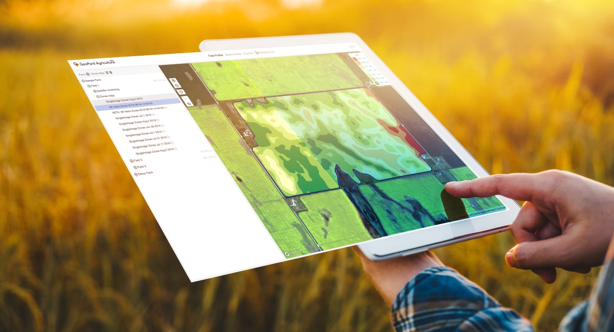
Precision agriculture relies on spatial variability data to prescribe site-specific inputs. Vegetation index maps produced from drone or satellite imagery reveal the within-field variability in crop performance that average field measurements obscure.

These maps feed directly into variable-rate application systems, allowing farmers to apply more fertilizer where the crop needs it and less where it does not, reducing costs and environmental impact simultaneously.

Growth Stages of Maize Where Vegetation Indices Are Most Useful

“The right index at the right growth stage unlocks crop intelligence that blanket scouting simply cannot provide — and the timing of that data collection is as important as the index chosen.”

1. Emergence Stage

At emergence, plant cover is sparse and soil dominates the image. Standard NDVI performs poorly here because the soil background noise overwhelms the weak canopy signal. Soil-adjusted indices like SAVI and MSAVI are the appropriate tools during this phase.

They apply a correction factor to reduce the influence of exposed soil on the index value, allowing meaningful measurements of plant density and early establishment uniformity.

2. Vegetative Growth (V Stages)

From V3 through V12, the maize canopy expands rapidly. This is the most critical window for nitrogen management, as the crop’s demand for nitrogen accelerates sharply.

NDRE and CI Green are the most responsive indices during this period because the red edge band detects subtle reductions in chlorophyll before NDVI’s broader signal changes. UAV flights at V6 and V10 timed with side-dress nitrogen decisions produce the highest return on data investment.

Growth Stages of Maize Where Vegetation Indices Are Most Useful

3. Tasseling and Silking

Tasseling (VT) and silking (R1) are the most yield-sensitive stages in the entire maize life cycle. Canopy closure is near-complete at this point, which means NDVI and EVI can now read the full canopy without soil interference.

Both indices peak around VT in healthy crops. Any plateau or early decline in index values at this stage is a reliable indicator of stress that will translate into kernel abortion and yield loss.

4. Grain Filling

During grain fill (R3–R5), the primary management concern shifts to water stress and disease. NDWI (Normalized Difference Water Index, calculated from NIR and SWIR bands) and thermal indices complement the standard suite during this phase by detecting canopy water content reductions that precede visible wilting.

NDVI values begin to decline naturally as the crop matures, so interpreting index trajectories requires benchmarking against the expected seasonal pattern for the hybrid being grown.

5. Maturity

At physiological maturity (R6), all major vegetation indices decline as the canopy senesces and chlorophyll degrades. Index data at maturity is primarily used for retrospective analysis — correlating seasonal VI trajectories with actual harvest yield data to validate prediction models and improve future season benchmarks. Time-series analysis of index curves from emergence through maturity provides the richest data foundation for building field-specific yield models.

Common Vegetation Indices Used for Maize Growth Monitoring

1. NDVI (Normalized Difference Vegetation Index)

NDVI is the most widely used vegetation index in agriculture. It measures the contrast between NIR and red reflectance and is calculated as:

NDVI = (NIR − Red) / (NIR + Red)

NDVI values range from −1 to +1. Healthy, dense maize canopies typically score between 0.7 and 0.9 at peak greenness. Its best applications include tracking canopy development from V6 through tasseling, identifying underperforming field zones, and correlating with LAI and above-ground biomass.

NDVI’s key limitation is saturation in dense canopies — once LAI exceeds roughly 3 m²/m², additional leaf area produces diminishing changes in the NDVI signal, reducing sensitivity at peak canopy.

A 2024 study published in Agriculture (MDPI), using UAV-based NDVI monitoring across two growing seasons in Hungary, found that the strongest NDVI-to-yield correlation occurred at the post-silking stage (R = 0.638 in 2023 and R = 0.634 in 2024), confirming NDVI’s reliability as an in-season yield indicator at that specific growth window.

2. GNDVI (Green NDVI)

GNDVI replaces the red band with the green band: GNDVI = (NIR − Green) / (NIR + Green). The green channel is more sensitive to chlorophyll concentration than the red channel, making GNDVI better at detecting moderate chlorophyll variation in mature, dense canopies where NDVI has saturated.

Its primary application in maize is nitrogen status assessment during mid-vegetative and reproductive stages. Research published in ScienceDirect (2024) confirmed that GNDVI, when combined with NDRE in multi-index regression models, substantially improved maize yield prediction accuracy, particularly at pre-flowering stages.

3. EVI (Enhanced Vegetation Index)

EVI improves on NDVI by incorporating the blue band and applying atmospheric correction coefficients: EVI = 2.5 × [(NIR − Red) / (NIR + 6 × Red − 7.5 × Blue + 1)]. This formula simultaneously reduces atmospheric noise and soil background interference, making EVI more sensitive than NDVI in dense canopy conditions where NDVI saturates.

EVI is the preferred index for monitoring maize canopy structure from tasseling through early grain fill when plant cover is near complete. It is a core index in MODIS satellite products and is widely used for regional-scale maize monitoring.

A study in Agriculture (2024) using MODIS MOD09A1 data over Jilin Province, China, found that combining multiple vegetation indices including EVI with a shape model significantly improved phenological stage detection accuracy across key maize growth periods compared to single-index approaches.

For large-scale regional crop monitoring, fusing EVI with other indices in time-series models delivers more reliable phenological tracking than any single index alone.

4. SAVI (Soil Adjusted Vegetation Index)

SAVI introduces a soil brightness correction factor (L) into the NDVI formula: SAVI = [(NIR − Red) / (NIR + Red + L)] × (1 + L), where L = 0.5 for typical soil conditions. By dampening the reflectance contribution of bare soil, SAVI produces more accurate canopy measurements at early maize growth stages when ground cover is less than 50%. It is the standard choice for monitoring plant establishment, stand uniformity, and early-season vigor from emergence through V4.

5. NDRE (Normalized Difference Red Edge)

NDRE uses the red edge and NIR bands: NDRE = (NIR − Red Edge) / (NIR + Red Edge). The red edge band sits in a spectral region where small changes in chlorophyll concentration produce large reflectance changes, making NDRE more sensitive than NDVI to nitrogen-driven chlorophyll variation.

A study published in Sensors (2024) using UAV photogrammetry at an LSU AgCenter research station found that NDRE at 87 days after planting predicted maize grain yield with an R² of 0.9097, an exceptionally strong relationship that underlines NDRE’s value for late-season nitrogen management and yield forecasting.

6. MSAVI (Modified Soil Adjusted Vegetation Index)

MSAVI improves on SAVI by making the L factor dynamic rather than fixed, so it adjusts automatically to the degree of vegetation cover: MSAVI = [2 × NIR + 1 − √((2 × NIR + 1)² − 8 × (NIR − Red))] / 2.

This self-adjustment makes MSAVI more accurate than SAVI across the full range of canopy development from bare-soil emergence through full cover at tasseling. It requires no assumption about soil brightness, making it more transferable across different field conditions and soil types.

7. VARI (Visible Atmospherically Resistant Index)

VARI uses only visible bands (Red, Green, Blue): VARI = (Green − Red) / (Green + Red − Blue). Its value lies in being computable from standard RGB cameras — the type carried by most commercial drones at low cost.

While VARI lacks the nitrogen and biomass sensitivity of multispectral indices, it provides a usable first-pass assessment of canopy greenness, making it accessible to farmers who do not yet have multispectral sensor capability.

Research published in ScienceDirect (2025) confirmed VARI as one of the useful VI inputs in machine learning models for maize yield prediction across varied growing environments.

8. OSAVI (Optimized Soil Adjusted Vegetation Index)

OSAVI is a simplified version of SAVI with a fixed L value of 0.16, optimized for partial canopy cover conditions: OSAVI = (NIR − Red) / (NIR + Red + 0.16).

This specific L value was empirically determined to minimize soil background effects across a wide range of vegetation densities. OSAVI performs well from V2 through V6, bridging the gap between SAVI’s early-season utility and NDVI’s peak-season accuracy.

9. CI Green (Chlorophyll Index Green)

CI Green estimates chlorophyll content directly from reflectance: CI Green = (NIR / Green) − 1. Because chlorophyll is the primary nitrogen-storage pigment in leaves, CI Green tracks the canopy’s nitrogen status without requiring the red edge band.

This makes it valuable when only a standard green band is available, such as from Sentinel-2 imagery, and it performs reliably from V6 through silking for mid-season nitrogen management decisions.

10. CI Red Edge (Chlorophyll Index Red Edge)

CI Red Edge replaces the green band with the red edge band: CI Red Edge = (NIR / Red Edge) − 1. This substitution makes it significantly more sensitive to chlorophyll changes than CI Green, particularly in the mid-to-late vegetative stages when the canopy is dense enough that the green band signal begins to saturate. CI Red Edge is one of the best-performing indices for detecting subtle nitrogen gradients across field management zones in maize.

Comparing Vegetation Indices for Maize Monitoring

1. Best Index for Early Growth

SAVI and MSAVI consistently outperform NDVI and EVI during early maize development (emergence through V4) because they reduce soil background noise that would otherwise dominate the index signal when canopy cover is below 40%. OSAVI offers a useful intermediate option when soil conditions are variable across a field.

Comparing Vegetation Indices for Maize Monitoring

2. Best Index for Nitrogen Detection

NDRE and CI Red Edge are the strongest indices for detecting nitrogen deficiency in maize. Both exploit the red edge band’s high sensitivity to chlorophyll concentration. At the V6 to V10 stage — the most critical window for nitrogen application decisions — these indices detect deficiency 7 to 14 days before NDVI shows any measurable response, providing a significant lead time for corrective action.

3. Best Index for Biomass Estimation

NDVI and EVI are the most validated indices for above-ground dry biomass estimation in maize. Research using UAV multispectral imagery combined with texture features in PMC (2023) found that vegetation indices based on the red (650 nm), red-edge (705 nm), and NIR (842 nm) bands showed the highest correlations with LAI — a closely related proxy for biomass accumulation during the vegetative period.

4. Best Index for Dense Canopies

EVI is the preferred index when the maize canopy has closed fully, typically from tasseling through early grain fill. Where NDVI saturates above an LAI of approximately 3, EVI continues to respond to additional leaf area and chlorophyll variation because its atmospheric and soil correction terms prevent signal saturation at high biomass levels.

5. Best Index for Drought Stress

NDWI (NIR and SWIR-based water index) and NDVI used together are the most effective combination for drought stress detection in maize. NDWI tracks tissue water content changes directly, while NDVI captures the secondary effect of water stress on canopy greenness. Multispectral sensors that include SWIR capability add the most value here, though these sensors remain more expensive than standard five-band multispectral systems.

Applications of Vegetation Indices in Maize Production

A vegetation index is only as useful as the decision it enables — the goal is always to convert spectral data into a field action that improves yield, reduces cost, or both.

1. Biomass Estimation

NDVI and EVI values correlate strongly with above-ground dry biomass across the maize vegetative period. Repeated UAV flights or satellite overpasses at two-week intervals generate biomass accumulation curves that reveal whether a field is tracking toward its yield potential or falling behind the expected growth trajectory for a given season.

2. Chlorophyll Measurement

CI Green and CI Red Edge provide non-destructive canopy-level chlorophyll estimates that track the crop’s photosynthetic capacity. Research published in PMC (2024) using UAV-based SPAD (chlorophyll meter reading) estimation in maize confirmed that the modified red-edge ratio index achieved an R² of 0.87 for predicting leaf chlorophyll content at the middle growth stage, demonstrating the practical accuracy that red-edge indices deliver for this application.

3. Nitrogen Status Assessment

Nitrogen is the nutrient that most directly limits maize yield, and its status fluctuates throughout the season as the crop’s demand changes. A 2025 study published in Frontiers in Plant Science integrated Sentinel-2A satellite imagery, UAV multispectral data, and ground observations across four maize growth stages in 2024 and developed a novel regional-scale nitrogen content inversion model using multiple vegetation indices combined with band correction.

The framework achieved high validation accuracy across 48 independent sampling points, demonstrating how satellite-UAV fusion expands the scalability of VI-based nitrogen management beyond individual fields to farm and regional scales.

4. Water Stress Detection

Water stress in maize first reduces stomatal conductance, then leaf water content, and finally green biomass — three processes that affect different spectral bands in sequence. Early-stage water stress shows in thermal band data and SWIR-based indices before NDVI declines.

Monitoring the combination of NDWI and NDVI across the grain fill period — when water stress has the greatest yield impact — allows irrigation scheduling to be based on actual crop demand rather than calendar-based rules.

5. Disease Monitoring

Fungal diseases like northern corn leaf blight and gray leaf spot change the spectral signature of infected leaves before large lesions are visible to the human eye. Infected tissue shows a characteristic drop in NIR reflectance and a shift in red edge position.

Multi-temporal VI monitoring allows detection of localized spectral anomalies that indicate emerging disease pressure, enabling targeted fungicide application rather than field-wide spraying.

6. Pest Damage Detection

Defoliation from pest feeding reduces LAI, which directly lowers NDVI and EVI values in affected patches. Armyworm infestations, for example, create characteristic spatial patterns of index decline that are detectable from drone imagery before the infestation spreads to neighboring field sections.

High-resolution UAV flights (ground sampling distance below 5 cm) provide the spatial detail needed to distinguish insect damage from other causes of canopy variation.

7. Yield Estimation

Vegetation index values measured at specific critical growth stages — particularly V12, VT, and R3 — are reliable predictors of final grain yield when combined with historical yield maps and weather data. Multi-index fusion approaches consistently outperform single-index models.

The combination of GNDVI, NDRE, and SCCCI (Simplified Canopy Chlorophyll Content Index) around pre-flowering has shown particularly strong yield forecasting accuracy in published maize research from ScienceDirect (2026).

Research across two growing seasons in Hungary found correlation coefficients of 0.638 and 0.634 between post-silking NDVI and final grain yield. Multi-index models including NDRE and GNDVI push prediction accuracy higher still.

8. Variable Rate Fertilizer Application

VI-based canopy maps generated from drone flights are used directly to build prescription maps for variable-rate nitrogen applicators. Fields are divided into management zones based on index values, and each zone receives a nitrogen dose calibrated to its specific crop demand.

Remote sensing and variable-rate technology together accounted for 58% of the precision farming technology market share in 2025 (Precedence Research, 2026), reflecting how central this workflow has become to commercial maize production.

A 2025 study in Agriculture (MDPI) found that moderate nitrogen doses of 120–180 kg ha⁻¹ provided the optimal nutrition level for maize, increasing yield by up to 5.086 t ha⁻¹ compared to unfertilized controls, with NDVI-based monitoring proving effective not just for yield optimization but specifically for guiding site-specific fertilization strategies.

NDVI-based nitrogen management at the post-silking stage (when VI-yield correlation peaks) can replace traditional soil-test-only fertilization approaches and significantly improve both input efficiency and grain yield.

Platforms Used to Collect Vegetation Index Data

1. Satellite Imagery

Satellites like Sentinel-2 (10 m resolution, 5-day revisit) and Planet Labs satellites (3 m resolution, daily revisit) provide consistent, weather-permitting spectral data across large areas at low per-hectare cost.

Sentinel-2’s inclusion of red edge bands (B5, B6, B7 at 705, 740, 783 nm) makes it particularly valuable for NDRE and CI Red Edge calculations across regional maize monitoring programs. The limitation is cloud cover: a cloudy period during a critical growth window can produce data gaps that interrupt temporal monitoring.

2. Drone-Based Remote Sensing

Fixed-wing and multi-rotor drones equipped with multispectral cameras provide field-scale imagery at resolutions of 2–10 cm per pixel. This level of detail resolves individual plant rows, allowing within-row variation in canopy health to be measured.

Drone surveys can be scheduled on demand, regardless of satellite overpass timing, making them ideal for capturing data at exact agronomic decision points such as side-dress nitrogen application or irrigation scheduling windows.

3. UAV Multispectral Cameras

Multispectral cameras such as the MicaSense RedEdge, Parrot Sequoia, and DJI Zenmuse P1 capture imagery in five or more narrow spectral bands simultaneously, including red, green, blue, red edge, and NIR.

These systems include a calibrated reflectance panel and a sunshine sensor to normalize data for varying light conditions during a flight, which is essential for producing accurate, reproducible index values rather than relative comparisons.

4. Handheld Crop Sensors

Active optical sensors like the GreenSeeker and CropCircle emit their own light source and measure the reflectance of individual plants at close range, eliminating the effect of variable sunlight.

These sensors are used for rapid in-field nitrogen status assessment at specific sampling points. Their data complements drone and satellite imagery by providing ground truth measurements that validate the remote sensing index values at known locations.

5. Tractor-Mounted Sensors

Tractor-mounted active sensors, such as the John Deere Hagie and Trimble GreenSeeker RT, scan the maize canopy continuously as the tractor moves through the field and feed real-time NDVI data directly into a variable-rate controller. This closed-loop system allows fertilizer rate adjustments to be made on the go, based on live crop condition data, without a separate data processing step between sensing and application.

Factors Affecting Vegetation Index Accuracy in Maize Fields

1. Soil Background

Exposed soil has its own spectral signature that blends with the plant canopy signal, particularly when cover is below 50%. Soil-adjusted indices (SAVI, MSAVI, OSAVI) are designed to minimize this effect, but soil color, moisture, and organic matter content still influence index values in early-season imagery. Calibrating index thresholds for specific soil types in a region improves interpretation accuracy.

2. Cloud Cover

Clouds block solar radiation and cause variable shadowing on the ground, making reflectance measurements unreliable for passive sensors on satellites and drones.

Active sensors are immune to cloud cover because they supply their own illumination. Cloud cover is the single most important factor limiting the utility of satellite-based VI monitoring in regions with high cloud frequency during the growing season.

Factors Affecting Vegetation Index Accuracy in Maize Fields

3. Sun Angle

Low sun angles increase shadow fraction within the canopy, artificially depressing NIR reflectance and distorting index values. UAV flights conducted between 10 AM and 2 PM local solar time minimize shadow effects and produce more consistent data. Consistency in flight time across repeat surveys is as important as absolute timing, because it allows meaningful comparison between dates.

4. Crop Density

Plant population directly affects canopy closure and therefore how quickly VI values rise from planting through canopy closure. Fields with lower plant populations close the canopy later, which prolongs the period during which soil background interferes with index readings. Population maps obtained from emergence imagery allow VI thresholds to be adjusted for local density variation.

5. Growth Stage

The same VI value means different things at different growth stages. An NDVI of 0.5 at V6 may indicate a healthy, well-developing canopy, while an NDVI of 0.5 at VT would signal significant stress.

Interpreting VI values without accounting for growth stage leads to misclassification of crop condition. Time-series analysis, which compares current values against expected seasonal curves, corrects for this by contextualizing each reading within the crop’s developmental trajectory.

6. Sensor Resolution

Coarser-resolution sensors mix the spectral signals of crop, soil, and field edges within a single pixel — a problem called “mixed pixels.” At Sentinel-2’s 10 m resolution, a single pixel covers 100 m² of ground, which often includes multiple crop rows and inter-row soil.

Higher-resolution drone imagery (5 cm per pixel) eliminates mixed pixels and provides a much purer canopy spectral signal, at the cost of increased data volume and processing time.

Limitations of Vegetation Indices for Maize Monitoring

1. Saturation in Dense Canopies

NDVI, the most widely used index, saturates at LAI values above approximately 3 m²/m², which maize typically reaches by V10. Above this threshold, additional increases in canopy greenness or biomass produce negligible changes in NDVI. EVI, GNDVI, and NDRE are designed to address this limitation but require more spectral bands than NDVI and are not always available from lower-cost sensors.

2. Weather Dependency

Passive remote sensing systems depend on consistent solar illumination. Cloud cover, haze, and atmospheric aerosols absorb and scatter incoming solar radiation before it reaches the crop and again on the way back to the sensor, distorting reflectance values.

Atmospheric correction algorithms applied during data processing reduce but do not eliminate this effect. In tropical maize production regions with prolonged cloudy seasons, data gaps can be frequent enough to compromise time-series monitoring.

3. Mixed Pixels

At low spatial resolutions, pixels capture signals from both the crop canopy and the soil, roads, irrigation equipment, or field margins. The resulting mixed-pixel reflectance produces index values that do not represent the canopy alone. Field boundary masking and the use of the highest-feasible spatial resolution sensor are standard practices to minimize this error.

4. Calibration Requirements

Producing accurate, reproducible index values requires radiometric calibration of the sensor, correction for atmospheric effects, and normalization for variable illumination during drone flights. Skipping these steps produces relative VI maps that cannot be compared between dates or across fields, limiting their usefulness for time-series monitoring and multi-field benchmarking.

5. Need for Ground Truth Validation

Vegetation indices are indirect measurements. They estimate crop properties — chlorophyll, nitrogen, biomass — by correlating spectral patterns with biological variables rather than measuring them directly.

Every VI-based crop assessment benefits from ground truth validation: physical measurements of leaf nitrogen, chlorophyll meter readings, or destructive biomass samples taken at a representative subset of locations across the field. Ground truth data anchors the remote sensing interpretation and prevents misdiagnosis.

Best Practices for Using Vegetation Indices in Maize Fields

1. Choosing the Right Index

Index selection should follow the monitoring objective and the available sensor. For nitrogen assessment, choose NDRE or CI Red Edge if a red edge band is available. For early-season stand assessment, use SAVI or MSAVI.

For peak-season canopy monitoring and yield forecasting, use EVI or NDVI combined with GNDVI or NDRE. Avoid using NDVI alone in early season or at high canopy density — its limitations in both scenarios are well established.

2. Selecting the Right Growth Stage

Timing data collection to agronomic decision points maximizes the management value of VI data. A practical monitoring schedule for maize would include:

  1. V2–V4 (emergence check): Use SAVI or MSAVI to assess stand uniformity and identify replanting zones.
  2. V6 (side-dress nitrogen decision): Use NDRE or CI Red Edge to map nitrogen status and generate variable-rate prescription.
  3. V10–V12 (canopy closure): Use NDVI and EVI to assess biomass and flag underperforming management zones.
  4. VT (tasseling): Use NDVI and GNDVI to evaluate canopy peak and identify areas at risk of stress during pollination.
  5. R3 (milk stage): Use NDVI and NDWI to detect water stress and assess grain fill progress.
  6. R6 (maturity): Use index data to correlate seasonal VI trajectory with harvest yield for model calibration.

3. Combining Multiple Indices

No single index captures the full complexity of maize crop condition. Combining two or more indices that target different biological signals produces richer diagnostic maps. The combination of NDRE for nitrogen status, NDVI for overall biomass, and NDWI for water content covers the three most common limiting factors in maize production. Multi-index fusion within machine learning models delivers measurably higher yield prediction accuracy than any single-index approach.

4. Integrating Ground Observations

VI maps should always be interpreted alongside field scouting observations. When a VI anomaly appears in a drone map, a physical field visit to that location confirms whether the spectral signal reflects a real agronomic problem — nitrogen deficiency, compaction, waterlogging, pest damage — or an artifact of sensor noise, shadow, or soil variation. Ground observations also provide the training data needed to calibrate local VI thresholds for specific hybrids, soils, and management systems.

5. Using Time-Series Analysis

A single VI image is a snapshot. A time-series of images from emergence through maturity is a story. Plotting index values over time reveals growth trajectories that identify stress events by the date they occurred, how severe they were, and how long they lasted. Time-series data also enables comparison between the current season and historical benchmarks, providing context that single-date imagery cannot deliver.

Future Trends in Maize Growth Monitoring

1. Artificial Intelligence

AI algorithms are increasingly being applied to vegetation index data to automate interpretation tasks that currently require an agronomist’s judgment. Deep learning models trained on large VI datasets can classify stress type, severity, and spatial extent from multispectral imagery in seconds, flagging action-required zones for agronomist review rather than requiring a full manual analysis of every image.

The AI in agriculture market was valued at USD 2.1 billion in 2023 and is projected to grow at a CAGR of over 24% through 2032 (GMI, 2025), reflecting how rapidly this capability is being commercialized.

2. Machine Learning Models

Random Forest, XGBoost, and convolutional neural networks (CNNs) applied to multi-index, multi-temporal datasets are consistently outperforming traditional regression-based VI-yield models.

Research using GBM (Gradient Boosting Machines) for maize yield prediction achieved R² values of 0.78 when integrating VI time-series with meteorological data, outperforming simpler regression approaches.

These models learn complex, non-linear relationships between spectral patterns and agronomic outcomes that linear models cannot capture.

3. Hyperspectral Imaging

Hyperspectral sensors capture reflectance data across hundreds of narrow spectral bands simultaneously, compared to the five to ten bands of typical multispectral cameras. This spectral density enables the detection of crop stress signals that fall in narrow spectral windows invisible to broadband sensors.

Hyperspectral indices for disease detection, heavy metal stress, and micronutrient deficiency are actively being validated for maize, with commercial UAV hyperspectral systems becoming increasingly affordable.

4. Real-Time Crop Monitoring

The combination of sensor miniaturization, satellite constellation expansion, and 5G connectivity is driving toward real-time crop condition monitoring — where VI data is available continuously during the growing season rather than weekly or bi-weekly.

Planet Labs’ daily satellite revisit rate and the deployment of IoT-enabled field sensors that stream data to cloud platforms already provide near-real-time monitoring capability for early adopters.

DJI’s drone-based remote sensing systems have reported a 67.78% reduction in chemical input volumes when prescription maps derived from VI data feed variable-rate spraying systems (Mordor Intelligence, 2026).

5. Integration with Precision Agriculture Systems

The next step in maize VI monitoring is seamless integration between data capture, processing, interpretation, and field action. Cloud-based farm management platforms are already connecting satellite and drone imagery pipelines directly to variable-rate controller software, reducing the time from data capture to field action from days to hours.

As APIs between imagery providers, agronomic software, and farm equipment become standardized, the workflow from “drone flight” to “variable-rate prescription applied” will become accessible to producers at all scales.

Frequently Asked Questions

Which vegetation index is best for maize?
No single index is universally best. NDRE performs best for nitrogen assessment, SAVI for early-stage monitoring, EVI for dense canopy conditions, and NDVI for general biomass and yield correlation. Combining two or three indices tailored to the monitoring objective consistently outperforms any single index.

How often should vegetation indices be monitored?
For full-season maize management, a monitoring interval of every 7 to 14 days during the V4 to R3 period is recommended. Critical decision windows (V6 for nitrogen, VT for stress assessment, R3 for irrigation) justify flights or satellite data pulls regardless of the standard monitoring schedule.

Which vegetation index works best during early maize growth?
SAVI and MSAVI perform best from emergence through V4 because they reduce the influence of exposed soil on the index value, producing meaningful canopy measurements even when ground cover is below 30%.

Can vegetation indices detect disease before symptoms appear?
Research indicates that foliar diseases alter the spectral signature of infected leaves before visible lesions appear. Red edge-based indices are the most sensitive for early disease detection because they respond to chlorophyll degradation in infected tissue. Detection lead time depends on disease type and severity, but early detection of 5 to 10 days before visual symptoms has been demonstrated in controlled studies.

Conclusion

Vegetation indices for maize growth monitoring have moved well beyond research curiosity. They are now practical, field-tested tools that give farmers and agronomists the ability to see crop stress, nitrogen deficiency, and yield-limiting conditions weeks before those problems become visible — and before they cause irreversible yield loss. Selecting the right index for each growth stage is not a minor technical detail; it is the difference between detecting a real problem and generating misleading data. Combining multiple indices — NDRE for nitrogen, EVI for dense-canopy biomass, NDWI for water status — delivers a diagnostic picture that no single measurement can provide. Integrating that spectral picture with physical field observations grounds the data in agronomic reality and prevents the misinterpretation that comes from relying on remote sensing alone.
Role of Deployment-Aware NAS for Efficient UAV-Based Crop Monitoring

Unmanned Aerial Vehicles (UAVs), or drones, are transforming modern agriculture by providing fast, aerial views of fields. They are used to scan crops for health, growth stage, pests, weeds, and yield estimation. For example, China now has over 250,000 agricultural drones in operation, and in Thailand about 30% of farmland was covered by drone spraying or monitoring by 2023. These UAVs make farming more efficient by quickly detecting problems (like pest outbreaks or water stress) that can be missed on the ground.

However, small UAVs have very limited onboard computing power and battery life. Running complex AI vision algorithms on them in real time is therefore a challenge. Traditional lightweight object detection models (like tiny YOLO or MobileNet-based detectors) can only partially meet these needs: they often sacrifice accuracy or speed and require significant manual tuning. This gap motivates deployment-aware Neural Architecture Search (NAS): an automated design method that tailors deep learning models to the exact requirements of field-deployed UAVs.

Modern precision agriculture uses UAVs (drones) to survey fields and monitor crop conditions. By flying over large areas, drones can collect high-resolution images of plants, soil, and field patterns. These images are fed to computer vision algorithms that detect weeds among crops, estimate yield (e.g. counting fruits or heads), or spot early signs of disease or nutrient deficiency. For instance, drones allow targeted herbicide spraying on weed patches, reducing chemical use and costs.

However, the small on-board computers in drones (often limited to a few watts of power) struggle to run large neural networks at flight speed. This makes it hard to do real-time analysis: if a drone sees a problem, it needs to react quickly or log the data before battery runs out. Current lightweight detectors (e.g. YOLOv8 nano, YOLO-tiny, MobileNets) are designed by hand and often involve trade-offs: making a model smaller speeds it up, but can hurt accuracy.

As a result, there is a strong need for methods that automatically find the best possible model given the UAV’s constraints. Deployment-aware NAS fits this need by searching for neural network architectures that jointly optimize detection accuracy and resource usage (latency, power, memory) under real UAV conditions. This approach can deliver specialized models that run efficiently on drone hardware yet remain highly accurate for crop monitoring tasks.

UAV Object Detection Requirements in Crop Monitoring

Agricultural UAVs perform a range of visual detection tasks, each with its own demands:

1. Crop health and stress detection: Drones use RGB, thermal or multispectral cameras to identify stressed plants, nutrient deficiencies, or disease symptoms. Real-time algorithms can map field variability, guiding irrigation or fertilization. Accurate detection of plant stress signs allows timely interventions to save yield.

2. Weed identification: Detecting weeds among crops lets farmers spray only unwanted plants, saving herbicide. For example, a study on cotton fields used UAV imagery with a YOLOv7-based detector and achieved about 83% accuracy at separating weeds from cotton. Yet distinguishing visually similar weeds and crops remains hard in cluttered field images.

UAV Object Detection Requirements in Crop Monitoring

3. Pest and disease detection: UAVs can spot outbreaks (e.g. locusts, insects, or fungal blight) earlier than humans on foot. Drones also support mapping pest-infested zones via multispectral imaging, which improves on RGB alone. Rapid, accurate pest detection is critical to prevent spread.

4. Yield estimation: Counting fruits, heads of grain, or plants from the air helps predict harvest volumes. Models trained to detect apples, melons, or wheat heads on UAV images can accelerate yield estimation. For example, neural networks on drone images have been used to count watermelon and melon crops in fields.

5. Surveying and mapping: Drones also create field maps (topography, soil differences) that help plan cultivation. Though not strictly object detection, this forms part of UAV monitoring.

These tasks often demand near-real-time inference: a drone flying over fields may need to process video frames on-the-fly (several frames per second) so that control decisions (like adjusting altitude or activating a sprayer) can be made immediately. In other cases, slight delays (seconds) might be acceptable if data are logged and analyzed after landing.

Importantly, UAV vision must handle environmental variability: bright sunlight, shadows, wind-induced motion blur, occlusion by overlapping leaves, or changes in altitude and angle. Object sizes vary (close-up weeds vs. distant pest clusters), so detectors must manage multi-scale features.

Finally, agricultural UAV missions involve strict trade-offs among accuracy, latency, and energy. High detection accuracy is needed to avoid missing weeds or pests, but running a very deep network can drain the battery quickly. A detection model must therefore be fast and energy-efficient while still accurate enough for the task. These stringent requirements highlight why specialized model design is needed for UAVs in agriculture.

Lightweight Object Detectors for UAV Platforms

Lightweight object detectors are neural networks specifically designed to run on limited hardware. They often use small backbones (like MobileNet or ShuffleNet), reduced layer widths, or simplified neck/head designs. For example, YOLO family models include “nano” and “tiny” versions (e.g. YOLOv8n, YOLOv5s) that have fewer parameters and require fewer operations (FLOPs).

Such detectors can run at tens of frames per second on embedded hardware like NVIDIA Jetson Nano or Google Coral. For instance, Ag-YOLO was a custom YOLO-based detector for palm plantations that ran at 36.5 fps on an Intel Neural Compute Stick 2 (using only 1.5 W) and achieved high accuracy (F1 = 0.9205). This model used about 12× fewer parameters than YOLOv3-Tiny while doubling its speed.

Lightweight Object Detectors for UAV Platforms

These examples show the trade-offs in model design: reducing a model’s size or complexity (e.g. fewer layers or channels) typically speeds up inference and lowers energy use, but can reduce accuracy. Ag-YOLO sacrificed some capacity to gain speed and efficiency, yet still maintained a high F1 score of 0.92 on its task.

Similarly, three YOLOv7 variants were compared for weed detection: the full YOLOv7 achieved 83% accuracy, while a smaller YOLOv7-w6 net dropped to 63% accuracy. This illustrates a limitation of generic lightweight detectors: models tuned for one environment or object type may underperform on another. A detector slimmed down for speed might miss subtle cues (e.g. small or camouflaged weeds), hurting robustness under varying conditions.

In agriculture, these generic lightweight networks may not be optimal without further adjustment. For example, a YOLOv7 model pre-trained on common datasets might not handle the unique textures and scales of crop imagery perfectly. Hence, there is a need for task- and platform-specific optimization of the model architecture. Manual tuning (changing layers, filters, etc.) for each new drone type or crop variety is labor-intensive. This motivates automated methods—such as deployment-aware NAS—to find the best balance of size, accuracy, and robustness for a given UAV platform and agricultural application.

Neural Architecture Search in UAV-Based Vision Systems

Neural Architecture Search (NAS) is an automated method for designing neural network architectures. Instead of manually setting the number of layers, filters, and connections, NAS uses algorithms (reinforcement learning, evolutionary methods, or gradient-based search) to explore a space of possible designs and find ones that optimize a chosen objective (like accuracy).

NAS has already been applied to create mobile-friendly networks. For example, Google’s MnasNet was a pioneering “platform-aware” NAS that directly included real device latency in the objective. MnasNet measured inference time on a Google Pixel phone for each candidate model during search, and balanced accuracy against this measured latency. The result was a family of CNNs that were both fast and accurate on mobile hardware, outperforming manually designed MobileNets and NASNet models on ImageNet.

However, generic NAS approaches like MnasNet focus on general vision tasks (ImageNet classification or COCO detection) and general hardware (e.g. mobile phones). For UAV crop monitoring, the problem is more specialized. We want detectors optimized for specific object classes (plants, weeds, pests) and tailored to the UAV’s sensors and flight profile. A standard NAS that optimizes only for accuracy or generic latency may overlook nuances like small-object detection or energy constraints.

Also, traditional NAS methods can be very computationally expensive (often requiring days on large GPU clusters), which is not always practical for agriculture researchers. Therefore, task-specific NAS frameworks are needed for UAV vision. These must incorporate UAV-relevant criteria and be as efficient as possible.

In all cases, constraint-awareness is critical: the NAS must be aware of the target device constraints (similar to MnasNet) and the real-time demands of in-flight UAV tasks. If search is too slow or ignores energy use, the resulting model may not actually work well in the field.

In practice, NAS for UAV vision would include hardware latency and energy directly in the search metric. For example, one could measure a candidate detector’s frame rate on the actual drone computer (like an NVIDIA Jetson) and use that as a score. This is in contrast to using simple proxies like FLOPs, which don’t capture real-world speed.

By doing so, the NAS can discover architectures that best exploit the device’s capabilities. In summary, NAS offers a way to automatically design detectors for UAVs, but it must be adapted to consider UAV-specific tasks and efficiency requirements.

Deployment-Aware NAS: Core Principles

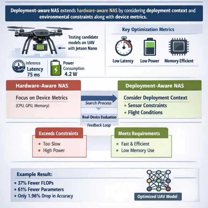
Deployment-aware NAS extends hardware-aware NAS by including deployment context and environmental constraints in the design process. In other words, it not only accounts for the drone’s hardware (CPU/GPU speed, memory limits, energy budget) but also for what the UAV will actually encounter in the field. This means explicitly optimizing for metrics like inference latency on the target device, power consumption, and memory footprint, all while still seeking high detection accuracy.

For instance, during NAS one could deploy each candidate model on a Jetson Nano attached to the UAV and record its real-world inference time and energy use. This empirical feedback helps guide the search toward models that truly meet the deployment criteria.

Deployment-Aware NAS: Core Principles

Hardware-aware NAS (like MnasNet) focuses on device metrics, whereas deployment-aware NAS goes further: it may consider sensor input characteristics (e.g. image resolution, multispectral channels) and application latency targets (frames per second needed). It can even incorporate flight constraints like maximum allowable memory or include evaluations under simulated wind shake or motion blur.

A deployment-aware NAS might penalize architectures that exceed, say, 5W power draw or that need more memory than the drone has. By doing so, the search naturally biases toward practical models for the UAV’s field operation. In essence, deployment-aware NAS is about closing the loop between model design and real-world use. Rather than choosing an architecture in isolation and hoping it works, it systematically includes real-device testing during search.

For example, Kerec et al. (2026) used such a framework to search for a UAV detector: they built on a YOLOv8n baseline but included Jetson Nano latency and energy in the search. The resulting model had 37% fewer GFLOPs and 61% fewer parameters than YOLOv8n, with only a 1.96% drop in mAP. This clearly shows how deployment constraints steered the NAS to a much lighter, faster network.

Role of Deployment-Aware NAS in Precision Agriculture Monitoring

Deployment-aware NAS can greatly improve UAV crop monitoring by tailoring detectors to agricultural conditions. For example, a search can favor architectures that excel at detecting small, thin objects (like narrow weeds or thin corn seedlings) or at distinguishing plants from soil backgrounds. It can adjust network depth and receptive fields to the typical flying height: at low altitude, objects fill the image and may require fine detail, whereas at higher altitude the network should be good at small-scale detection. A deployment-aware NAS can encode these requirements into its search space.

Speed is critical in the field. Imagine a drone detects a pest outbreak; if the model is fast enough to process video at, say, 30 fps, it can alert the pilot or trigger an immediate treatment action. In tests, a NAS-designed model ran 28% faster on a Jetson Nano than the standard YOLOv8n, thanks to its optimized architecture. It also used 18.5% less energy under ONNX runtime, meaning the drone can fly longer on the same battery. These gains make in-flight decision-making more feasible and extend mission duration.

Robustness is another benefit. Since deployment-aware NAS involves actual device evaluation, the search can include tests under varied conditions. For instance, it might simulate low-light or include training images from dawn and dusk, ensuring the final detector maintains accuracy under real weather and lighting changes. The work demonstrated that the NAS-derived detector generalized well: they tested it on two different crop datasets (wheat heads and cotton seedlings) and found strong performance across both.

Role of Deployment-Aware NAS in Precision Agriculture Monitoring

This suggests that deployment-aware NAS helped find common, useful features for agriculture, improving generalization to new fields. Overall, deployment-aware NAS helps balance accuracy with longer flight time. By cutting computation, drones use less power and can cover more area per battery charge, all while still detecting crops and pests reliably.

Search Space Design for Agricultural UAV Detectors

An important part of deployment-aware NAS is the search space – the set of possible network designs it considers. For UAV crop detectors, the search space can be crafted to include promising architectures for this domain. Key parts include:

1. Backbone design: The backbone is the feature extractor. For UAVs, one might include lightweight convolutional building blocks such as depthwise separable convolutions (as used in MobileNet), or inverted residual blocks. Inverted residuals and linear bottlenecks (MobileNetV2 style) are well-known for mobile efficiency. The search space could allow varying the width (number of channels) and depth of each block to match the UAV’s compute budget. Attention or transformer-inspired modules might also be included if the UAV can afford them at low power.

2. Neck design: Many object detectors use feature pyramids (FPN) or path aggregation networks to combine multiscale features. The search could explore simplified FPNs or lightweight feature aggregation. For example, using a single-scale head vs. multi-scale heads could be options. The space might allow pooling layers or skip connections that help detect objects at different sizes.

3. Head design: The detection head (classification and box regression layers) can also be varied. For UAVs looking at uniform fields, a simpler head might suffice. But to catch small weeds, the search might include extra convolutional layers or different anchor schemes.

4. Lightweight operations: The search space can explicitly allow only low-cost operations. For instance, choosing between a 3×3 conv versus a cheaper 1×3+3×1 factorized conv, or including GhostNet modules. It can also allow small kernel sizes or reduced dimensions to limit computation. All these choices are driven by the hardware. The space may forbid any layer configuration that exceeds the drone’s memory limit or expected energy threshold.

By carefully designing this search space, the NAS process is guided toward effective yet efficient architectures. The result might be a novel combination of blocks not considered in standard models. The best-found detector used custom block choices that cut GFLOPs by 37% and parameters by 61% compared to YOLOv8n.

This was possible because the NAS could mix and match backbone and head elements under the UAV constraints. In summary, the search space for agricultural UAV detectors focuses on scalable, lightweight building blocks and multi-scale handling, all within the limits of the onboard hardware.

Optimization Objectives and Constraints

Deployment-aware NAS must juggle multiple objectives. The primary goal is usually detection accuracy (e.g. mean Average Precision, mAP), as measured on crop monitoring datasets. For example, mAP@50 (accuracy at 50% IOU) is a common metric. The NAS-optimized model had only a 1.96% drop in mAP@50 compared to the base YOLOv8n, a very small loss for the gains achieved. Precision and recall (or F1 score) on key classes (weeds, crops) are also considered.

At the same time, latency and energy must be optimized. Latency is the inference time per image; for an embedded GPU it might be 20–50 ms or more. Lower latency means higher frame rates. Energy consumption (joules per frame) is crucial for flight endurance. Memory footprint (number of parameters, model size) is another constraint; models must fit into the device’s RAM. Therefore, NAS usually sets a target or penalty for these constraints.

For example, any model slower than a certain threshold or above a parameter budget might be downranked. This effectively turns NAS into a multi-objective optimization problem: maximize accuracy while minimizing latency, energy, and size.

Practically, this could be done by a weighted sum of objectives or by hard constraints. Some methods give a large penalty to any candidate exceeding the UAV’s power limit. Others explicitly compute an energy metric: models were tested under ONNX runtime to measure “energy efficiency,” and the best model was +18.5% more energy-efficient than YOLOv8n. This was one of the objectives guiding their search.

The trade-offs found can be visualized on a Pareto frontier: at one end, extremely fast small models with lower accuracy; at the other, large accurate models that are too slow or power-hungry for a drone. Deployment-aware NAS aims to find a sweet spot on this frontier that matches the real mission priorities (e.g. slight accuracy loss for a big speedup). In sum, the NAS must consider accuracy metrics (mAP, F1) and inference constraints (ms per frame, joules per frame, memory) together. This balanced optimization is what makes a model truly deployment-ready for UAV use.

Training and Evaluation in Realistic Agricultural Settings

For the NAS-found detectors to work well, they must be trained and tested on realistic agricultural data. This means using datasets that capture the variability of real fields: different crop species, growth stages, seasons, lighting conditions, and altitudes. For example, training on images of only young corn shoots may not generalize to mature wheat heads. Field-representative datasets ensure the model learns features that matter on the farm. Data augmentation (random crops, brightness changes, motion blur) can also be applied during training to mimic drone motion and lighting.

Training and Evaluation in Realistic Agricultural Settings

When evaluating, it’s important to test the model in as-real conditions as possible. Simulation tools can help (e.g. flying virtual drone over 3D fields) but real flight tests are the gold standard. Onboard benchmarking is performed by running the model on the actual UAV hardware. After NAS they deployed the candidate on a Jetson Nano and measured 28.1% faster inference (compared to baseline YOLOv8n) and better energy use. This kind of real-device feedback confirms that the search produced a model that truly meets the requirements.

Generalization is also crucial. A model might be searched and trained on one crop (say, wheat), but farmers need detectors that work across fields. The study demonstrated strong cross-crop generalization: the NAS-derived detector trained on one task still performed well on a different crop dataset (cotton seedlings) without retraining. This suggests that deployment-aware NAS can yield robust architectures. However, domain shifts (e.g. moving from cornfields to orchards) may still require fine-tuning or further search. Cross-season testing (summer vs. autumn imagery) is also advised.

Finally, every new model should be benchmarked on the UAV platform prior to deployment. This includes logging its accuracy and speed on drones, ensuring it doesn’t overheat the hardware, and verifying power draw. Only then can farmers trust it for mission-critical monitoring. By combining field-relevant training and rigorous hardware evaluation, deployment-aware NAS yields detectors that are not only theoretically efficient, but proven in the field.

Benefits Over Manually Designed UAV Detectors

Deployment-aware NAS offers several clear advantages over traditional, manually designed models for UAVs:

1. Better performance trade-offs: The NAS-found models tend to provide higher accuracy-speed-energy efficiency combinations. For example, the best model ran 28% faster and used 18.5% less energy on Jetson Nano than the manually chosen YOLOv8n baseline, while losing only ~2% in detection mAP. Achieving such a balance by hand would be very difficult.

2. Improved generalization: Models discovered by NAS can be more adaptable to new conditions, since the search can incorporate diverse data or objectives. The automatically designed detector generalized well across different crop types (wheat and cotton) and lighting conditions. This broad robustness is crucial when flights encounter unexpected scenes.

3. Reduced engineering effort: NAS automates a lot of trial-and-error. Instead of manually tweaking layer sizes and testing many candidates, a deployment-aware NAS iteratively explores choices and finds the best design for you. This saves development time and expertise, making it easier to update detectors for new tasks or hardware.

4. Scalability: Once set up, the NAS framework can be used for different UAV platforms or missions. For instance, the same deployment-aware NAS could search for a detector tuned to a different camera resolution or drone model by simply changing the constraint inputs. This is much more scalable than redesigning networks from scratch for each scenario.

Challenges and Limitations

Deployment-aware NAS is powerful but not a magic bullet. It must be applied thoughtfully, with awareness of its resource demands and the variability of the target environment. Despite its promise, deployment-aware NAS has challenges:

1. High search cost: NAS can require substantial computation. Even with efficient algorithms, searching architecture space can take many GPU hours (or specialized compute). If not carefully managed, the search overhead could be prohibitive for some teams.

2. Data bias and domain shift: The NAS is only as good as the data used. If training images are not representative of field conditions, the found architecture may underperform in reality. For example, a model tuned on one crop type or one geographic region might not transfer perfectly to another without further adaptation.

3. Hardware heterogeneity: UAV hardware comes in many flavors (different embedded GPUs, CPUs, FPGAs). A model optimized for one board may not be optimal on another. Deployment-aware NAS must either rerun searches for each platform or use conservative constraints that fit all – which can limit performance.

4. Practical constraints: Real farming deployments involve issues like network updates over the air, system integration with flight control, and safety certification. Even the best NAS model must be integrated into a full drone system. Coordinating model updates, regulatory approvals, and farmer training are non-technical hurdles.

Future Directions

The future will likely see even tighter integration of model design, sensor tech, and UAV control. Deployment-aware NAS will remain a key tool in this co-design process.Looking ahead, several exciting avenues emerge:

1. Online and adaptive NAS: Instead of a one-time offline search, future systems might adjust the network in real-time or between flights. For example, a drone could start with a base model and, using lightweight NAS algorithms, tweak itself to handle new lighting or terrain conditions on the fly. This “on-device NAS” is very challenging but could greatly improve adaptability.

2. Co-design of sensors and models: Future precision agriculture systems could jointly optimize the choice of camera (RGB, multispectral, infrared) and the neural network. Deployment-aware NAS could extend to include sensor parameters (like spectral bands used) in its search, finding the best combination of hardware and model.

3. Multispectral/hyperspectral integration: As the cotton disease study suggests, integrating multispectral imagery can boost detection, especially of early-stage problems. Future NAS could explore multi-stream models that fuse RGB and near-infrared channels to detect subtle plant changes more reliably.

4. Autonomous decision pipelines: Ultimately, NAS-optimized detectors may feed into full autonomy. For example, a drone might automatically generate a spray plan or alert farm managers if it detects certain conditions. Deployment-aware NAS could be extended to end-to-end pipelines (detection + action models), optimizing the whole system.

5. Ethical and environmental considerations: As UAVs become more capable, we must consider privacy, airspace safety, and impacts on farm labor (as noted by Agrawal & Arafat). Ensuring NAS-optimized drones are used responsibly in agriculture is an important future goal.

Conclusion

Deployment-aware NAS represents a powerful approach to tailor lightweight object detectors for UAV-based crop monitoring. By embedding UAV hardware and mission constraints into the search, it produces models that save computation and energy without sacrificing much accuracy. For example, recent work showed a NAS-designed detector using 37% fewer FLOPs and 61% fewer parameters than the reference YOLOv8n, yet its mAP dropped by only ~2%.

On actual drone hardware, this meant 28% faster inference and 18% better energy efficiency. Such gains translate to longer flight times, faster analysis, and more responsive agriculture support. Compared to manually crafted models, deployment-aware NAS delivers better performance generalization, less manual tuning effort, and scalability to new UAV platforms.

In the context of precision agriculture, these improvements can make UAV crop monitoring more practical and effective. Drones equipped with NAS-optimized detectors can more reliably spot weeds, pests, or stress, enabling timely interventions that save resources and increase yields. As agriculture continues to adopt drones and AI, deployment-aware NAS will play a central role in ensuring the models running on those drones are efficient, accurate, and field-ready. It bridges the gap between cutting-edge neural network research and the practical needs of farmers, helping to drive the future of data-driven, precision farming.

Barley Farming Gets a Boost With Lightweight YOLOv5 Detection

Highland barley, a resilient cereal crop grown in the high-altitude regions of China’s Qinghai-Tibet Plateau, plays a critical role in local food security and economic stability. Known scientifically as Hordeum vulgare L., this crop thrives in extreme conditions—thin air, low oxygen levels, and an average annual temperature of 6.3°C—making it indispensable for communities in harsh environments.

With over 270,000 hectares dedicated to its cultivation in China, primarily in the Xizang Autonomous Region, highland barley accounts for more than half of the region’s planted area and over 70% of its total grain production. Accurate monitoring of barley density—the number of plants or spikes per unit area—is essential for optimizing agricultural practices, such as irrigation and fertilization, and predicting yields.

However, traditional methods like manual sampling or satellite imaging have proven inefficient, labor-intensive, or insufficiently detailed. To address these challenges, researchers from Fujian Agriculture and Forestry University and Chengdu University of Technology developed an innovative AI model based on YOLOv5, a cutting-edge object-detection algorithm.

Their work, published in Plant Methods (2025), achieved remarkable results, including a 93.1% mean average precision (mAP)—a metric measuring overall detection accuracy—and a 75.6% reduction in computational costs, making it suitable for real-time drone deployments.

Challenges and Innovations in Crop Monitoring

The importance of highland barley extends beyond its role as a food source. In 2022 alone, Rikaze City, a major barley-producing region, harvested 408,900 tons of barley across 60,000 hectares, contributing nearly half of Tibet’s total grain output.

Despite its cultural and economic significance, estimating barley yields has long been challenging. Traditional methods, such as manual counting or satellite imagery, are either too labor-intensive or lack the resolution needed to detect individual barley spikes—the grain-bearing part of the plant, which are often just 2–3 centimeters wide.

Manual sampling requires farmers to physically inspect sections of a field—a process that is slow, subjective, and impractical for large-scale farms. Satellite imagery, while useful for broad observations, struggles with low resolution (often 10–30 meters per pixel) and frequent weather disruptions, such as cloud cover in mountainous regions like Tibet.

To overcome these limitations, researchers turned to unmanned aerial vehicles (UAVs), or drones, equipped with 20-megapixel cameras. These drones captured 501 high-resolution images of barley fields in Rikaze City during two critical growth stages: the growth stage in August 2022, characterized by green, developing spikes, and the maturation stage in August 2023, marked by golden-yellow, harvest-ready spikes.

Drone-Based Barley Field Monitoring in Rikaze City

However, analyzing these images posed challenges, including blurred edges caused by drone motion, the small size of barley spikes in aerial views, and overlapping spikes in densely planted fields.

To address these issues, researchers preprocessed the images by splitting each high-resolution image into 35 smaller sub-images and filtering out blurry edges, resulting in 2,970 high-quality sub-images for training. This preprocessing step ensured the model focused on clear, actionable data, avoiding distractions from low-quality regions.

Technical Advancements in Object Detection

Central to this research is the YOLOv5 algorithm (You Only Look Once version 5), a one-stage object-detection model known for its speed and modular design. Unlike older two-stage models like Faster R-CNN, which first identify regions of interest and then classify objects, YOLOv5 performs detection in a single pass, making it significantly faster.

The baseline YOLOv5n model, with 1.76 million parameters (configurable components of the AI model) and 4.1 billion FLOPs (floating-point operations, a measure of computational complexity), was already efficient. However, detecting tiny, overlapping barley spikes required further optimization.

The research team introduced three key enhancements to the model: depthwise separable convolution (DSConv), ghost convolution (GhostConv), and a convolutional block attention module (CBAM).

Depthwise separable convolution (DSConv) reduces computational costs by splitting the standard convolution process—a mathematical operation that extracts features from images—into two steps. First, depthwise convolution applies filters to individual color channels (e.g., red, green, blue), analyzing each channel separately.

This is followed by pointwise convolution, which combines results across channels using 1×1 kernels. This approach slashes parameter counts by up to 75%.

Parameter Reduction in Depthwise Separable Convolution

For example, a traditional 3×3 convolution with 64 input and 128 output channels requires 73,728 parameters, while DSConv reduces this to just 8,768—an 88% reduction. This efficiency is critical for deploying models on drones or mobile devices with limited processing power.

Ghost convolution (GhostConv) further lightens the model by generating additional feature maps—simplified representations of image patterns—through simple linear operations, such as rotation or scaling, instead of resource-heavy convolutions.

Traditional convolution layers produce redundant features, wasting computational resources. GhostConv addresses this by creating “ghost” features from existing ones, effectively halving the parameters in certain layers.

For instance, a layer with 64 input and 128 output channels would traditionally require 73,728 parameters, but GhostConv reduces this to 36,864 while maintaining accuracy. This technique is especially useful for detecting small objects like barley spikes, where computational efficiency is paramount.

The convolutional block attention module (CBAM) was integrated to help the model focus on critical features, even in cluttered environments. Attention mechanisms, inspired by human visual systems, allow AI models to prioritize important parts of an image.

CBAM employs two types of attention: channel attention, which identifies important color channels (e.g., green for growing spikes), and spatial attention, which highlights key regions within an image (e.g., clusters of spikes). By replacing standard modules with DSConv and GhostConv and incorporating CBAM, the researchers created a leaner, more precise model tailored for barley detection.

Implementation and Results

To train the model, researchers manually labeled 135 original images using bounding boxes—rectangular frames marking the location of barley spikes—categorizing spikes into growth and maturation stages. Data augmentation techniques—including rotation, noise injection, occlusion, and sharpening—expanded the dataset to 2,970 images, improving the model’s ability to generalize across diverse field conditions.

For example, rotating images by 90°, 180°, or 270° helped the model recognize spikes from different angles, while adding noise simulated real-world imperfections like dust or shadows. The dataset was split into a training set (80%) and a validation set (20%), ensuring robust evaluation.

Training took place on a high-performance system with an AMD Ryzen 7 CPU, NVIDIA RTX 4060 GPU, and 64GB RAM, using the PyTorch framework—a popular tool for deep learning. Over 300 training epochs (complete passes through the dataset), the model’s precision (accuracy of correct detections), recall (ability to find all relevant spikes), and loss (error rate) were meticulously tracked.

The results were striking. The improved YOLOv5 model achieved a precision of 92.2% (up from 89.1% in the baseline) and a recall of 86.2% (up from 83.1%), outperforming the baseline YOLOv5n by 3.1% in both metrics. Its mean average precision (mAP)—a comprehensive metric averaging detection accuracy across all categories—reached 93.1%, with individual scores of 92.7% for growth-stage spikes and 93.5% for maturation-stage spikes.

YOLOv5 Model Training Results

Equally impressive was its computational efficiency: the model’s parameters dropped by 70.6% to 1.2 million, and FLOPs decreased by 75.6% to 3.1 billion. Comparative analyses with leading models like Faster R-CNN and YOLOv8n highlighted its superiority.

While YOLOv8n achieved a slightly higher mAP (93.8%), its parameters (3.0 million) and FLOPs (8.1 billion) were 2.5x and 2.6x higher, respectively, making the proposed model far more efficient for real-time applications.

Visual comparisons underscored these advancements. In growth-stage images, the improved model detected 41 spikes compared to the baseline’s 28. During maturation, it identified 3 spikes versus the baseline’s 2, with fewer missed detections (marked by orange arrows) and false positives (marked by purple arrows).

These improvements are vital for farmers relying on accurate data to predict yields and optimize resources. For instance, precise spike counts enable better estimates of grain production, informing decisions about harvest timing, storage, and market planning.

Future Directions and Practical Implications

Despite its success, the study acknowledged limitations. Performance dipped under extreme lighting conditions, such as harsh midday glare or heavy shadows, which can obscure spike details. Additionally, rectangular bounding boxes sometimes failed to fit irregularly shaped spikes, introducing minor inaccuracies.

The model also excluded blurry edges from UAV images, requiring manual preprocessing—a step that adds time and complexity.

Future work aims to address these issues by expanding the dataset to include images captured at dawn, noon, and dusk, experimenting with polygon-shaped annotations (flexible shapes that better fit irregular objects), and developing algorithms to better handle blurry regions without manual intervention.

The implications of this research are profound. For farmers in regions like Tibet, the model offers real-time yield estimation, replacing labor-intensive manual counts with drone-based automation. Distinguishing between growth stages enables precise harvest planning, reducing losses from premature or delayed harvesting.

Detailed data on spike density—such as identifying underpopulated or overcrowded areas—can inform irrigation and fertilization strategies, reducing water and chemical waste. Beyond barley, the lightweight architecture holds promise for other crops, such as wheat, rice, or fruits, paving the way for broader applications in precision agriculture.

Conclusion

In conclusion, this study exemplifies the transformative potential of AI in addressing agricultural challenges. By refining YOLOv5 with innovative lightweight techniques, the researchers have created a tool that balances accuracy and efficiency—critical for real-world deployment in resource-constrained environments.

Terms like mAP, FLOPs, and attention mechanisms may seem technical, but their impact is deeply practical: they enable farmers to make data-driven decisions, conserve resources, and maximize yields. As climate change and population growth intensify pressure on global food systems, such advancements will be indispensable.

For the farmers of Tibet and beyond, this technology represents not just a leap in agricultural efficiency, but a beacon of hope for sustainable food security in an uncertain future.

Reference: Cai, M., Deng, H., Cai, J. et al. Lightweight highland barley detection based on improved YOLOv5. Plant Methods 21, 42 (2025). https://doi.org/10.1186/s13007-025-01353-0

CMTNet Redefines Precision Agriculture By Outperforming Traditional Crop Classification

Accurate crop classification is essential for modern precision agriculture, enabling farmers to monitor crop health, predict yields, and allocate resources efficiently. Traditional methods, however, often struggle with the complexity of agricultural environments, where crops vary widely in type, growth stages, and spectral signatures.

What is Hyperspectral Imaging And CMTNet Framework?

Hyperspectral imaging (HSI), a technology that captures data across hundreds of narrow, contiguous wavelength bands, has emerged as a game-changer in this field. Unlike standard RGB cameras or multispectral sensors, which collect data in a few broad bands, HSI provides a detailed “spectral fingerprint” for each pixel.

For example, healthy vegetation strongly reflects near-infrared light due to chlorophyll activity, while stressed crops show distinct absorption patterns. By recording these subtle variations (from 400 to 1,000 nanometers) at high spatial resolutions (as fine as 0.043 meters), HSI enables precise differentiation of crop species, disease detection, and soil analysis.

Despite these advantages, existing techniques face challenges in balancing local details, like leaf texture or soil patterns, with global patterns, such as large-scale crop distribution. This limitation becomes especially apparent in noisy or imbalanced datasets, where subtle spectral differences between crops can lead to misclassifications.

To address these challenges, researchers developed CMTNet (Convolutional Meets Transformer Network), a novel deep learning framework that combines the strengths of convolutional neural networks (CNNs) and Transformers. CNNs are a class of neural networks designed to process grid-like data, such as images, using layers of filters that detect spatial hierarchies (e.g., edges, textures).

CMTNet Architecture and Performance

Transformers, originally developed for natural language processing, use self-attention mechanisms to model long-range dependencies in data, making them adept at capturing global patterns. Unlike earlier models that process local and global features sequentially, CMTNet uses a parallel architecture to extract both types of information simultaneously.

This approach has proven highly effective, achieving state-of-the-art accuracy on three major UAV-based HSI datasets. For instance, on the WHU-Hi-LongKou dataset, CMTNet reached an overall accuracy (OA) of 99.58%, outperforming the previous best model by 0.19%.

Challenges of Traditional Hyperspectral Imaging in Agricultural Classification

Early methods for analyzing hyperspectral data often focused on either spectral or spatial features, leading to incomplete results. Spectral techniques, such as principal component analysis (PCA), reduced the complexity of data by focusing on wavelength information but ignored spatial relationships between pixels.

PCA, for example, transforms high-dimensional spectral data into fewer components that explain the most variance, simplifying analysis. However, this approach discards spatial context, such as the arrangement of crops in a field. Conversely, spatial methods, like mathematical morphology operators, highlighted patterns in the physical layout of crops but overlooked critical spectral details.

Mathematical morphology uses operations like dilation and erosion to extract shapes and structures from images, such as the boundaries between fields. Over time, convolutional neural networks (CNNs) improved classification by processing both types of data.

However, their fixed receptive fields—the area of an image a network can “see” at once—limited their ability to capture long-range dependencies. For example, a 3D-CNN might struggle to distinguish between two soybean varieties with similar spectral profiles but different growth patterns across a large field.

Transformers, a type of neural network originally designed for natural language processing, offered a solution to this problem. By using self-attention mechanisms, Transformers excel at modeling global relationships in data. Self-attention allows the model to weigh the importance of different parts of an input sequence, enabling it to focus on relevant regions (e.g., a cluster of diseased plants) while ignoring noise (e.g., cloud shadows).

Yet, they often miss fine-grained local details, such as the edges of leaves or soil cracks. Hybrid models like CTMixer attempted to combine CNNs and Transformers but did so sequentially, processing local features first and global features later. This approach led to inefficient fusion of information and suboptimal performance in complex agricultural environments.

How CMTNet Works: Bridging Local and Global Features

CMTNet overcomes these limitations through a unique three-part architecture designed to extract and fuse spectral-spatial, local, and global features effectively.

1. The first component, the spectral-spatial feature extraction module, processes raw HSI data using 3D and 2D convolutional layers.

The 3D convolutional layers analyze both spatial (height × width) and spectral (wavelength) dimensions simultaneously, capturing patterns like the reflectance of specific wavelengths across a crop canopy. For example, a 3D kernel might detect that healthy corn reflects more near-infrared light in its upper leaves compared to lower ones.

The 2D layers then refine these features, focusing on spatial details like the arrangement of plants in a field. This two-step process ensures that both spectral diversity (e.g., chlorophyll content) and spatial context (e.g., row spacing) are preserved.

2. The second component, the local-global feature extraction module, operates in parallel. One branch uses CNNs to focus on local details, such as the texture of individual leaves or the shape of soil patches. These features are critical for identifying species with similar spectral profiles, such as different soybean varieties.

The other branch employs Transformers to model global relationships, such as how crops are distributed across large areas or how shadows from nearby trees affect spectral readings. By processing these features simultaneously rather than sequentially, CMTNet avoids the information loss that plagues earlier hybrid models.

For instance, while the CNN branch identifies the jagged edges of cotton leaves, the Transformer branch recognizes that these leaves are part of a larger cotton field bordered by sesame plants.

3. The third component, the multi-output constraint module, ensures balanced learning across local, global, and fused features. During training, separate loss functions are applied to each type of feature, forcing the network to refine all aspects of its understanding.

A loss function quantifies the difference between predicted and actual values, guiding the model’s adjustments. For example, the loss for local features might penalize the model for misclassifying leaf edges, while the global loss corrects errors in large-scale crop distribution.

These losses are combined using weights optimized through a random search—a technique that tests various weight combinations to maximize accuracy. This process results in a robust and adaptable model capable of handling diverse agricultural scenarios.

Evaluating CMTNet Performance on UAV Hyperspectral Datasets

To evaluate CMTNet, researchers tested it on three UAV-acquired hyperspectral datasets from Wuhan University. These datasets are widely used benchmarks in remote sensing due to their high quality and diversity:

  1. WHU-Hi-LongKou: This dataset covers 550 × 400 pixels with 270 spectral bands and a spatial resolution of 0.463 meters. A spatial resolution of 0.463 meters means each pixel represents a 0.463m × 0.463m area on the ground, allowing the identification of individual plants. It includes nine crop types, such as corn, cotton, and rice, with 1,019 training samples and 203,523 test samples.
  2. WHU-Hi-HanChuan: Capturing 1,217 × 303 pixels at 0.109-meter resolution, this dataset features 16 land cover types, including strawberries, soybeans, and plastic sheets. The higher resolution (0.109m) enables finer details, such as the distinction between young and mature soybean plants. Training and test samples totaled 1,289 and 256,241, respectively.
  3. WHU-Hi-HongHu: With 940 × 475 pixels and 270 bands, this high-resolution (0.043 meters) dataset includes 22 classes, such as cotton, rape, and garlic sprouts. At 0.043m resolution, individual leaves and soil cracks are visible, making it ideal for fine-grained classification. It contains 1,925 training samples and 384,678 test samples.

Comparison of High-Resolution Remote Sensing Datasets

The model was trained on NVIDIA TITAN Xp GPUs using PyTorch, with a learning rate of 0.001 and a batch size of 100. A learning rate determines how much the model adjusts its parameters during training—too high, and it may overshoot optimal values; too low, and training becomes sluggish.

Each experiment was repeated ten times to ensure reliability, and input patches—small segments of the full image—were optimized to 13 × 13 pixels through grid search, a method that tests different patch sizes to find the most effective.

CMTNet Achieves State-of-the-Art Accuracy in Crop Classification

CMTNet achieved remarkable results across all datasets, outperforming existing methods in both overall accuracy (OA) and class-specific performance. OA measures the percentage of correctly classified pixels across all classes, while average accuracy (AA) calculates the mean accuracy per class, addressing imbalances.

On the WHU-Hi-LongKou dataset, CMTNet achieved an OA of 99.58%, surpassing CTMixer by 0.19%. For challenging classes with limited training data, such as cotton (41 samples), CMTNet still reached 99.53% accuracy. Similarly, on the WHU-Hi-HanChuan dataset, it improved accuracy for watermelon (22 samples) from 82.42% to 96.11%, demonstrating its ability to handle imbalanced data through effective feature fusion.

Visual comparisons of classification maps revealed fewer fragmented patches and smoother boundaries between fields compared to models like 3D-CNN and Vision Transformer (ViT). For example, in the shadow-prone WHU-Hi-HanChuan dataset, CMTNet minimized errors caused by low sun angles, whereas ResNet misclassified soybeans as gray rooftops.

Performance of CMTNet on Various Datasets

Shadows pose a unique challenge because they alter spectral signatures—a soybean plant in shadow might reflect less near-infrared light, resembling non-vegetation. By leveraging global context, CMTNet recognized that these shadowed plants were part of a larger soybean field, reducing errors.

On the WHU-Hi-HongHu dataset, the model excelled in distinguishing spectrally similar crops, such as different brassica varieties, achieving 96.54% accuracy for Brassica parachinensis.

Ablation studies—experiments that remove components to assess their impact—confirmed the importance of each module. Adding the multi-output constraint module alone boosted OA by 1.52% on WHU-Hi-HongHu, highlighting its role in refining feature fusion. Without this module, local and global features were combined haphazardly, leading to inconsistent classifications.

Computational Trade-offs and Practical Considerations

While CMTNet’s accuracy is unmatched, its computational cost is higher than traditional methods. Training on the WHU-Hi-HongHu dataset took 1,885 seconds, compared to 74 seconds for Random Forest (RF), a machine learning algorithm that builds decision trees during training.

However, this trade-off is justified in precision agriculture, where accuracy directly impacts yield predictions and resource allocation. For example, misclassifying a diseased crop as healthy could lead to unchecked pest outbreaks, devastating entire fields.

For real-time applications, future work could explore model compression techniques, such as pruning redundant neurons or quantizing weights (reducing numerical precision), to reduce runtime without sacrificing performance. Pruning removes less important connections from the neural network, akin to trimming branches from a tree to improve its shape, while quantization simplifies numerical calculations, speeding up processing.

Future of Hyperspectral Crop Classification with CMTNet

Despite its success, CMTNet faces limitations. Performance dips slightly in heavily shadowed regions, as seen in the WHU-Hi-HanChuan dataset (97.29% OA vs. 99.58% in well-lit LongKou). Shadows complicate classification because they reduce the intensity of reflected light, altering spectral profiles.

Additionally, classes with extremely small training samples, like narrow-leaf soybean (20 samples), lag behind those with abundant data. Small sample sizes limit the model’s ability to learn diverse variations, such as differences in leaf shape due to soil quality.

Future research could integrate multimodal data, such as LiDAR elevation maps or thermal imaging, to improve resilience to shadows and occlusions. LiDAR (Light Detection and Ranging) uses laser pulses to create 3D terrain models, which could help distinguish crops from shadows by analyzing height differences.

Moreover, thermal imaging captures heat signatures, providing additional clues about plant health—stressed crops often have higher canopy temperatures due to reduced transpiration. Semi-supervised learning techniques, which leverage unlabeled data (e.g., UAV images without manual annotations), might also enhance performance for rare crop types.

By using consistency regularization—training the model to produce stable predictions across slightly altered versions of the same image—researchers can exploit unlabeled data to improve generalization.

Finally, deploying CMTNet on edge devices, like drones equipped with onboard GPUs, could enable real-time monitoring in remote fields. Edge deployment reduces reliance on cloud computing, minimizing latency and data transmission costs. However, this requires optimizing the model for limited memory and processing power, potentially through lightweight architectures like MobileNet or knowledge distillation, where a smaller “student” model mimics a larger “teacher” model.

Conclusion

CMTNet represents a significant leap forward in hyperspectral crop classification. By harmonizing CNNs and Transformers, it addresses long-standing challenges in feature extraction and fusion, offering farmers and agronomists a powerful tool for precision agriculture.

Applications range from real-time disease detection to optimizing irrigation schedules, all of which are critical for sustainable farming amid climate change and population growth. As UAV technology becomes more accessible, models like CMTNet will play a pivotal role in global food security.

Future advancements, such as lighter-weight architectures and multimodal data fusion, could further enhance their practicality. With continued innovation, CMTNet could become a cornerstone of smart farming systems worldwide, ensuring efficient land use and resilient food production for generations to come.

Reference: Guo, X., Feng, Q. & Guo, F. CMTNet: a hybrid CNN-transformer network for UAV-based hyperspectral crop classification in precision agriculture. Sci Rep 15, 12383 (2025). https://doi.org/10.1038/s41598-025-97052-w

Role of Deep Learning Computer Vision Applications for Early Plant Disease Detection

Plant diseases silently threaten global food security, destroying 10–16% of crops annually and costing the agriculture industry $220 billion in losses. Traditional methods like manual inspections and lab tests are slow, expensive, and often unreliable.

A groundbreaking 2025 study, “Deep Learning and Computer Vision in Plant Disease Detection” (Upadhyay et al.), reveals how AI plant disease detection and computer vision agriculture are transforming farming.

Why Early Plant Disease Detection Matters for Global Food Security

Agriculture employs 28% of the global workforce, with countries like India, China, and the U.S. leading crop production. Despite this, plant diseases caused by fungi, bacteria, and viruses slash yields and strain economies.

For instance, rice blast disease reduces harvests by 30–50% in affected regions, while citrus greening has wiped out 70% of Florida’s orange groves since 2005. Early detection is critical, but many farmers lack access to advanced tools or expertise.

This is where AI-driven disease detection steps in, offering fast, affordable, and precise solutions that outperform traditional methods.

How AI and Computer Vision Detect Crop Diseases

The study analyzed 278 research papers to explain how AI plant disease detection systems operate. First, cameras or sensors capture images of crops. These images are then processed using algorithms to identify signs of disease.

For example, RGB cameras take color photos to spot visible symptoms like leaf spots, while hyperspectral cameras detect hidden stress signals by analyzing hundreds of light wavelengths.

Once images are captured, they undergo preprocessing to enhance quality. Techniques like thresholding isolate diseased areas by color, and edge detection maps the boundaries of lesions or discoloration.

How AI and Computer Vision Detect Crop Diseases

Next, deep learning models analyze the preprocessed data. Convolutional Neural Networks (CNNs), the most common AI tools in agriculture, scan images layer by layer to identify patterns like unusual textures or colors.

In a 2022 trial, ResNet50—a popular CNN model—achieved 99.07% accuracy in diagnosing tomato diseases.

Meanwhile, Vision Transformers (ViTs) split images into patches and study their relationships, mimicking how humans analyze context. This approach helped detect grapevine vein-clearing virus with 71% accuracy in a 2020 study.

“The future of farming lies not in replacing humans, but in equipping them with intelligent tools.”

The Role of Advanced Sensors in Modern Farming

Different sensors offer unique advantages for precision agriculture. RGB cameras, though affordable and easy to use, struggle with early-stage diseases due to limited spectral detail. In contrast, hyperspectral cameras capture data across hundreds of light wavelengths, revealing stress signals invisible to the naked eye.

For example, researchers used hyperspectral imaging to diagnose apple valsa canker with 98% accuracy in 2022. However, these cameras cost 10,000–50,000, making them too expensive for small-scale farmers.

Thermal cameras provide another angle by measuring temperature changes caused by infections. A 2019 study found that leaves infected with citrus greening show distinct heat patterns, allowing early detection.

Meanwhile, multispectral cameras—a middle-ground option—track chlorophyll levels to assess plant health.

These sensors mapped wheat stripe rust in 2014, helping farmers target treatments more effectively. Despite their benefits, sensor costs and environmental factors like wind or uneven lighting remain challenges.

Public Datasets: The Backbone of AI Agriculture

Training reliable AI models requires vast amounts of labeled data. The PlantVillage dataset, a free resource with 87,000 images of 14 crops and 26 diseases, has become the gold standard for researchers.

Over 90% of studies cited in the paper used this dataset to train and test their models. Another key resource, the Cassava Disease Dataset, includes 11,670 images of cassava mosaic disease and achieved 96% accuracy with CNN models.

However, gaps persist. Rare diseases like pinewood nematode have fewer than 100 labeled images, limiting AI’s ability to detect them. Additionally, most datasets feature lab-captured images, which don’t account for real-world variables like weather or lighting.

To address this, projects like AI4Ag are crowdsourcing field images from farmers worldwide, aiming to build more robust and realistic datasets.

Measuring AI Performance: Accuracy, Precision, and Beyond

Performance Metrics of AI Plant Disease Detection Systems

Researchers use several metrics to evaluate AI plant disease detection systems. Accuracy—the percentage of correct diagnoses—ranges from 76.9% in early models to 99.97% in advanced systems like EfficientNet-B5.

However, accuracy alone can be misleading. Precision measures how many flagged diseases are real (avoiding false alarms), while recall tracks how many actual infections are detected.

For example, Mask R-CNN, an object-detection model, achieved 93.5% recall in spotting strawberry anthracnose but only 45% precision in cotton root rot detection.

The F1-Score balances precision and recall, offering a holistic performance view. In a 2023 trial, PlantViT—a hybrid AI model—scored 98.61% F1-Score on the PlantVillage dataset.

For object detection, mean Average Precision (mAP) is critical. Faster R-CNN, a popular model, achieved 73.07% mAP in apple disease trials, meaning it correctly located and classified infections in most cases.

Challenges Holding Back AI in Agriculture

Despite its potential, AI-driven disease detection faces hurdles. First, data scarcity plagues rare or emerging diseases.

  • For instance, only 20 images of cucumber powdery mildew were available for a 2021 study, limiting model reliability.
  • Second, environmental factors like wind, shadows, or varying light conditions reduce field accuracy by 20–30% compared to lab settings.
  • Third, high costs hinder adoption. Hyperspectral cameras, while powerful, remain unaffordable for small farmers, and AI tools require smartphones or internet access—still a barrier in rural areas.
  • Finally, trust issues persist. A 2023 survey found 68% of farmers hesitate to adopt AI due to its “black box” nature—they can’t see how decisions are made.

To overcome this, researchers are developing interpretable AI that explains diagnoses in simple terms, like highlighting infected leaf areas or listing symptoms.

The Future of Farming: 5 Innovations to Watch

1. Edge Computing for Real-Time Analysis: Lightweight AI models like MobileNetV2 (7 MB size) run on smartphones or drones, offering real-time disease detection without internet. In 2023, this model achieved 99.42% accuracy on potato disease classification, empowering farmers to make instant decisions.

2. Transfer Learning for Faster Adaptation: Pre-trained models like PlantViT can be fine-tuned for new crops with minimal data. A 2023 study adapted PlantViT for rice blast detection, achieving 87.87% accuracy using just 1,000 images.

3. Vision-Language Models (VLMs): Systems like OpenAI’s CLIP let farmers query AI using text (e.g., “Find brown spots on leaves”). This natural interaction bridges the gap between complex tech and everyday farming.

4. Foundation Models for General-Purpose AI: Large models like GPT-4 could simulate disease spread or recommend treatments, acting as virtual agronomists.

5. Collaborative Global Databases: Open-source platforms like PlantVillage and AI4Ag pool data from farmers and researchers worldwide, accelerating innovation.

Case Study: AI-Powered Mango Farming in India

In 2024, researchers developed a lightweight DenseNet model to combat mango diseases like anthracnose and powdery mildew. Trained on 12,332 field images, the model achieved 99.2% accuracy—higher than most lab-based systems.

With 50% fewer parameters, it runs smoothly on budget smartphones. Indian farmers now use a $10 app built on this AI to scan leaves and receive instant diagnoses, reducing pesticide use by 30% and saving crops.

Conclusion

AI plant disease detection and precision agriculture technology are reshaping farming, offering hope against food insecurity. By enabling early diagnosis, cutting chemical use, and empowering small farmers, these tools could boost global crop yields by 20–30%.

To realize this potential, stakeholders must address sensor costs, improve data diversity, and build farmer trust through education.

Reference: Upadhyay, A., Chandel, N.S., Singh, K.P. et al. Deep learning and computer vision in plant disease detection: a comprehensive review of techniques, models, and trends in precision agriculture. Artif Intell Rev 58, 92 (2025). https://doi.org/10.1007/s10462-024-11100-x

How UAS-Based High-Throughput Phenotyping is Transforming Modern Plant Breeding

By 2050, the global population is projected to reach 9.8 billion people, doubling the demand for food. However, expanding farmland to meet this need is unsustainable. Over 50% of new cropland created since 2000 has replaced forests and natural ecosystems, worsening climate change and biodiversity loss.

To avoid this crisis, scientists are turning to plant breeding—the science of developing crops with higher yields, disease resistance, and climate resilience. Traditional breeding methods, however, are too slow to keep up with the urgency of the problem.

This is where drones and artificial intelligence (AI) are stepping in as game-changers, offering a faster, smarter way to breed better crops.

Why Traditional Plant Breeding Is Falling Behind

Plant breeding relies on selecting plants with desirable traits, such as drought tolerance or pest resistance, and cross-breeding them over multiple generations. The biggest bottleneck in this process is phenotyping—the manual measurement of plant characteristics like height, leaf health, or yield.

For example, measuring plant height across a field of 3,000 plots can take weeks, with human errors causing inconsistencies of up to 20%. Additionally, crop yields are improving at just 0.5–1% annually, far below the 2.9% growth rate needed to meet 2050 demands.

Maize, a staple crop for billions, illustrates this slowdown: its annual yield growth has dropped from 2.2% in the 1960s to 1.33% today. To bridge this gap, scientists need tools that automate data collection, reduce errors, and speed up decision-making.

How Drone Technology Is Transforming Plant Breeding

Drones, or Unmanned Aerial Systems (UAS), equipped with advanced sensors and AI, are revolutionizing agriculture. These devices can fly over fields and collect precise data on thousands of plants in minutes, a process known as High Throughput Phenotyping (HTP).

Unlike traditional methods, drones capture data across entire fields, eliminating sampling bias. They use specialized sensors to measure everything from plant height to water stress levels.

For instance, multispectral sensors detect near-infrared light reflected by healthy leaves, while thermal cameras identify drought stress by measuring canopy temperature.

By automating data collection, drones reduce labor costs and accelerate breeding cycles, making it possible to develop improved crop varieties in years instead of decades.

The Science Behind Drone Sensors and Data Collection

Drones rely on a variety of sensors to gather critical plant data. RGB cameras, the most affordable option, capture visible light to measure canopy cover and plant height. In sugarcane fields, these cameras have achieved 64–69% accuracy in counting stalks, replacing error-prone manual counts.

Multispectral sensors go further by detecting non-visible wavelengths like near-infrared, which correlate with chlorophyll levels and plant health. For example, they have predicted drought tolerance in sugarcane with over 80% accuracy.

  • RGB Cameras: Capture red, green, and blue light to create color images.
  • Multispectral Sensors: Detect light beyond the visible spectrum (e.g., near-infrared).
  • Thermal Sensors: Measure heat emitted by plants.
  • LiDAR: Uses laser pulses to create 3D maps of plants.
  • Hyperspectral Sensors: Capture 200+ light wavelengths for ultra-detailed analysis.

Thermal sensors detect heat signatures, identifying water-stressed plants that appear hotter than healthy ones. In cotton fields, thermal drones have matched ground-based temperature measurements with less than 5% error.

LiDAR sensors use laser pulses to create 3D maps of crops, measuring biomass and height with 95% precision in energy cane trials. The most advanced tools, hyperspectral sensors, analyze hundreds of light wavelengths to spot nutrient deficiencies or diseases invisible to the naked eye.

These sensors helped researchers link 28 new genes to delayed aging in wheat, a trait that boosts yields.

From Flight to Insight: How Drones Analyze Crop Data

The drone phenotyping process begins with careful flight planning. Drones fly at 30–100 meters altitude, capturing overlapping images to ensure full coverage. A 10-hectare field, for instance, can be scanned in 15–30 minutes.

After the flight, software like Agisoft Metashape stitches thousands of images into detailed maps using Structure-from-Motion (SfM)—a technique that converts 2D photos into 3D models. These models allow scientists to measure traits like plant height or canopy cover at the tap of a button.

AI algorithms then analyze the data, predicting yields or identifying disease outbreaks. For example, drones scanned 3,132 sugarcane plots in just 7 hours—a task that would take three weeks manually. This speed and precision enable breeders to make faster decisions, such as discarding low-performing plants early in the season.

Key Applications of Drones in Modern Agriculture

Drones are being used to tackle some of farming’s biggest challenges. One major application is direct trait measurement, where drones replace manual labor. In maize fields, drones measure plant height with 90% accuracy, cutting errors from 0.5 meters to 0.21 meters.

They also track canopy cover, a metric indicating how well plants shade the ground to suppress weeds. Energy cane breeders used this data to identify varieties that reduce weed growth by 40%.

Another breakthrough is predictive breeding, where AI models use drone data to forecast crop performance. For instance, multispectral imagery has predicted maize yields with 80% accuracy, outperforming traditional genomic testing.

Drones also aid in gene discovery, helping scientists locate DNA segments responsible for desirable traits. In wheat, drones linked canopy greenness to 22 new genes, potentially boosting drought tolerance.

Additionally, hyperspectral sensors detect diseases like citrus greening weeks before symptoms appear, giving farmers time to act.

Boosting Genetic Gains with Precision Technology

Genetic gain—the annual improvement in crop traits due to breeding—is calculated using a simple formula:

(Selection Intensity × Heritability × Trait Variability) ÷ Breeding Cycle Time.

Genetic gain (ΔG) is calculated as:
ΔG = (i × h² × σp) / L

Where:

  • i = Selection intensity (how strict breeders are).
  •  = Heritability (how much of a trait is passed from parents to offspring).
  • σp = Trait variability in a population.
  • L = Time per breeding cycle.

Why It Matters: Drones improve all variables:

  1. i: Scan 10x more plants, allowing stricter selection.
  2. : Reduce measurement errors, improving heritability estimates.
  3. σp: Capture subtle trait variations across entire fields.
  4. L: Cut cycle time from 5 years to 2–3 years via early predictions.

Drones enhance every part of this equation. By scanning entire fields, they let breeders select the top 1% of plants instead of the top 10%, increasing selection intensity. They also improve heritability estimates by reducing measurement errors.

For example, manually assessing plant height introduces 20% variability, while drones cut this to 5%. Moreover, drones capture subtle trait variations across thousands of plants, maximizing trait variability.

Most importantly, they shorten breeding cycles by enabling early predictions. Sugarcane breeders using drones have tripled their genetic gains compared to traditional methods, proving the technology’s transformative potential.

Overcoming Challenges and Embracing the Future

Despite their promise, drone-based phenotyping still faces significant challenges. The high cost of advanced sensors remains a major barrier – hyperspectral cameras, for example, can exceed $50,000, making them unaffordable for most small-scale farmers.

Processing the massive amounts of data collected also requires substantial cloud computing resources, which adds to the expense. AI platforms like AutoGIS are automating data analysis, eliminating the need for manual input.

Researchers are also integrating drones with soil sensors and weather stations, creating a real-time monitoring system that alerts farmers to pests or droughts. These innovations are paving the way for a new era of precision agriculture, where data-driven decisions replace guesswork.

Conclusion

Drones and AI are not just transforming plant breeding—they’re redefining sustainable agriculture. By enabling faster development of drought-resistant, high-yield crops, these technologies could double food production by 2050 without expanding farmland.

This would save over 100 million hectares of forests, equivalent to the size of Egypt, and reduce the carbon footprint of farming. Farmers using drone data have already cut water and pesticide use by up to 30%, protecting ecosystems and lowering costs.

As one researcher noted, “We’re no longer guessing which plants are best. The drones tell us.” With continued innovation, this fusion of biology and technology could ensure food security for billions while safeguarding our planet.

Reference: Khuimphukhieo, I., & da Silva, J. A. (2025). Unmanned aerial systems (UAS)-based field high throughput phenotyping (HTP) as plant breeders’ toolbox: a comprehensive review. Smart Agricultural Technology, 100888.

How IoT Is Transforming Precision Agriculture and Solving Current Challenges?

The world’s population is growing rapidly, with estimates suggesting it will reach 9.7 billion by 2050. To feed everyone, food production must increase by 60%, but traditional farming methods—reliant on soil, heavy water use, and manual labor—are struggling to keep up.

Climate change, soil degradation, and water shortages are making matters worse. For instance, soil erosion alone costs farmers $40 billion annually in lost productivity, while traditional irrigation wastes 60% of freshwater due to outdated practices.

In India, unpredictable monsoons have reduced rice yields by 15% in the last decade. These challenges demand urgent solutions, and smart farming—powered by the Internet of Things (IoT) and aeroponics—offers a lifeline.

The Power of IoT in Modern Agriculture

At the heart of smart farming is IoT, a network of interconnected devices that collect and share data in real time. Wireless Sensor Networks (WSNs) are central to this system.
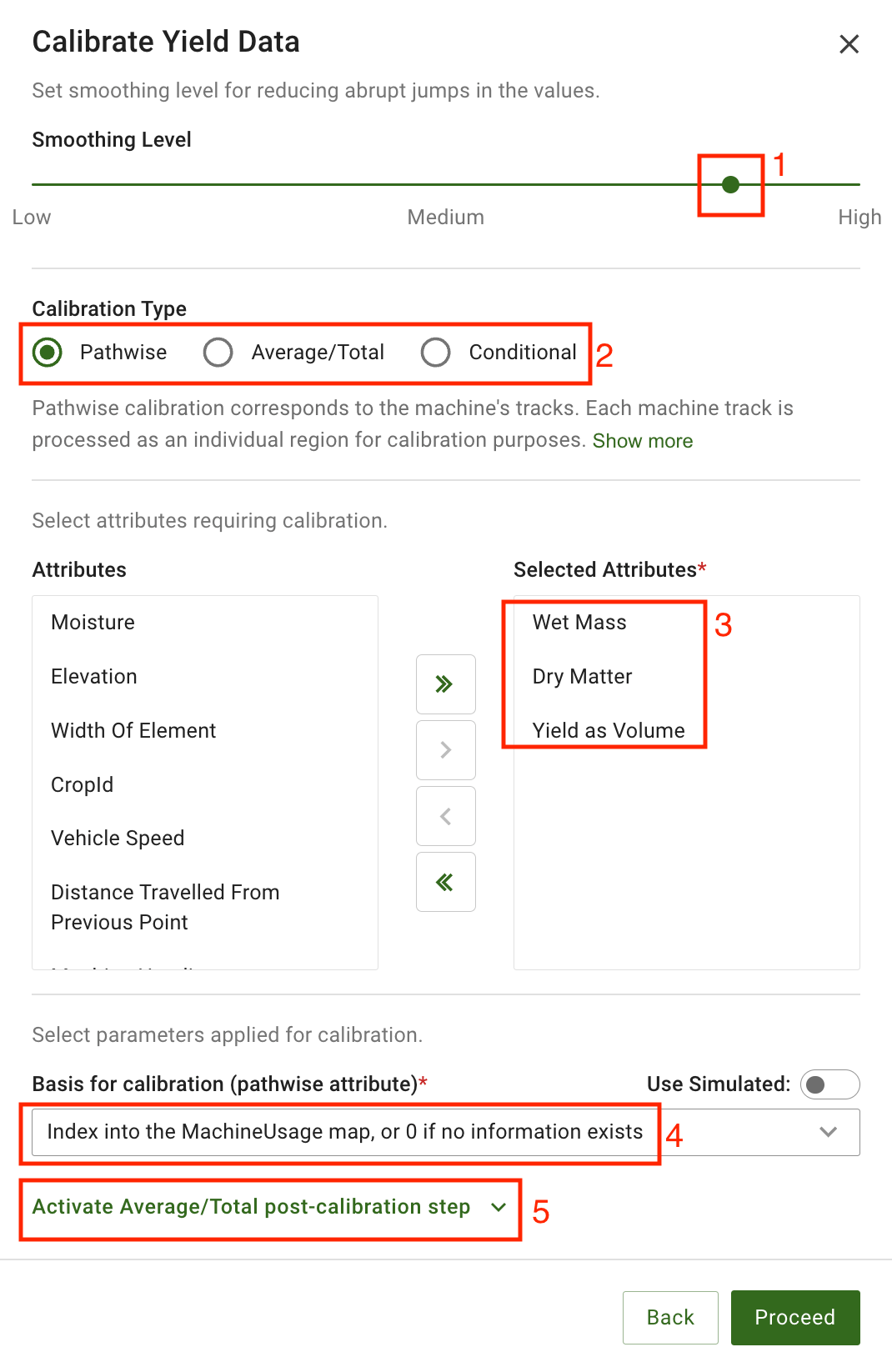
These networks use sensors placed in fields to monitor soil moisture, temperature, humidity, and nutrient levels. For example, the DHT22 sensor tracks humidity, while TDS sensors measure nutrient concentration in water.

This data is sent to cloud platforms like ThingSpeak or AWS IoT using low-power protocols like LoRa or ZigBee. Once analyzed, the system can trigger actions, such as turning on irrigation pumps or adjusting fertilizer levels.

In Coimbatore, India, a 2022 project demonstrated IoT’s potential. Sensors detected dry soil zones in tomato fields, enabling targeted irrigation that reduced water waste by 35%.

Similarly, drones equipped with multispectral cameras scan vast fields to identify issues like pest infestations or nutrient deficiencies.

A 2019 study used drones to detect Northern Leaf Blight in maize crops with 98% accuracy, saving farmers $120 per acre in losses. Machine learning further enhances these systems.

Researchers trained AI models on thousands of leaf images to diagnose diseases like powdery mildew with 99.53% accuracy, allowing farmers to act before crops are destroyed.

Aeroponics: Growing Food Without Soil

While IoT optimizes traditional farming, aeroponics reimagines agriculture entirely. This method grows plants in air, suspending their roots in mist-filled chambers that spray water and nutrients.

Unlike soil-based farming, aeroponics uses 95% less water and no pesticides. Roots absorb oxygen more efficiently, accelerating growth.

For example, lettuce grown aeroponically develops 65% faster than in soil, according to a 2018 study.

Aeroponics is especially valuable in cities or regions with poor soil. Vertical farms stack plants in towers, producing 10 times more food per square meter than traditional fields.

In Mexico City, a 2022 rooftop aeroponic farm yielded 3.8 kg of lettuce per square meter—triple the output of soil farming—while using just 10 liters of water per kilogram.

Singapore’s Sky Greens takes this further, growing 1 ton of vegetables daily in 30-foot towers, using 95% less land than conventional farms.

IoT takes aeroponics to the next level. Sensors monitor root chambers for humidity, pH, and nutrient levels, adjusting misting cycles automatically.

In a 2017 project, researchers automated an aeroponic system using Raspberry Pi, cutting labor costs by 50%. Farmers control these systems via mobile apps like AgroDecisor, which sends alerts for issues like nutrient imbalances.

Challenges Slowing Progress

Despite their potential, IoT and aeroponics face significant hurdles. High costs are a major barrier. A basic IoT setup costs 1,500 – 5,000, while advanced drones and sensors require 10,000–50,000 upfront—far beyond the reach of small-scale farmers in developing nations. Meanwhile, maintenance adds another 15–20% annually, straining budgets further.

Connectivity gaps compound the problem. About 40% of rural areas lack reliable internet, crippling real-time data transmission.

In Ethiopia, a 2021 IoT pilot failed when 3G signals dropped mid-field, disrupting irrigation schedules. Security risks also loom large. IoT protocols like MQTT and CoAP often lack encryption, leaving systems vulnerable to hackers.

In 2021, 62% of agricultural IoT systems reported cyberattacks, including data breaches that could manipulate sensor readings or disable equipment.

Technical complexity adds another layer of difficulty. Farmers need training to interpret data and troubleshoot systems.

A 2017 aeroponic project in Colombia collapsed when incorrect pH settings damaged crops, wasting $12,000 in seedlings.

Even power supply is an issue—solar sensors fail during monsoons, and drones last just 20–30 minutes per charge.

The Future of Farming: Innovations on the Horizon

Despite these challenges, the future looks promising. 5G networks will revolutionize connectivity, enabling drones to monitor vast farms in real time.

In Brazil, a 2023 trial used 5G-connected drones to scan 1,000+ acre soybean fields, detecting diseases in 10 minutes instead of days. Edge AI, which processes data directly on devices, reduces reliance on the cloud.

The MangoYOLO system, for instance, counts mangoes with 91% accuracy using onboard cameras, eliminating delays from data uploads.

Blockchain technology is another game-changer. By tracking produce from farm to consumer, it ensures transparency and reduces fraud.

The eFarm app uses crowdsourced data to verify organic certifications, cutting fraud by 30%. Walmart’s blockchain system reduced mango supply chain errors by 90% in 2022.

AI-driven greenhouses are also rising. These systems use models like VGG19 to monitor plant health with 91.52% accuracy.

In Japan, robots like AGROBOT harvest strawberries 24/7, tripling productivity. Urban areas are embracing aeroponics too—Berlin’s Infarm grows herbs in grocery stores, slashing transport emissions by 95%.

Governments and companies are stepping up. India’s 2023 Agri-Tech Initiative subsidizes IoT tools for 500,000 small farmers, while Microsoft’s FarmBeats provides low-cost drones to Kenyan farmers.

A Blueprint for Success

IoT and aeroponics are not just tools—they are essential for a sustainable future. By 2030, these technologies could:

  • Save 1.5 trillion liters of water annually.
  • Cut greenhouse gas emissions by 1.5 gigatons per year.
  • Feed 2 billion additional people without expanding farmland.

To achieve this, governments must subsidize affordable tools, expand rural internet access, and enforce cybersecurity standards. Farmers need training to harness these technologies effectively.

As the FAO states, “The future of food depends on today’s innovations.” By embracing IoT and aeroponics, we can cultivate a world where no one goes hungry—and where farming nurtures, rather than harms, our planet.

Reference: Dhanasekar, S. (2025). A comprehensive review on current issues and advancements of Internet of Things in precision agriculture. Computer Science Review, 55, 100694.

Remote Sensing Revolutionizes Nicotine Monitoring in Cigar Leaves

A groundbreaking study leverages UAV hyperspectral imaging and machine learning to accurately assess nicotine levels in cigar leaves.

Recent advancements in aerial hyperspectral imaging, combined with machine learning, have revolutionized nicotine monitoring in cigar leaves. This cutting-edge approach enhances assessment accuracy while providing valuable insights for the tobacco industry, where chemical composition is critical to quality.

Led by Tian et al. at Sichuan Agricultural University, researchers sought to overcome the limitations of traditional manual quality checks, which often lack precision and efficiency. Their study, published on February 2, 2025, identifies strong correlations between nitrogen fertilizer use, moisture levels, and nicotine concentrations, underscoring the importance of timely and precise monitoring techniques.

The study was conducted from May to September 2022 at the university’s Modern Agricultural Research Base, where researchers used unmanned aerial vehicles (UAVs) equipped with hyperspectral cameras to capture leaf reflectance spectra from 15 different cigar leaf varieties under various nitrogen treatments.

Their findings revealed a direct correlation between nitrogen fertilizer application and nicotine levels in cigar leaves. “With the increase in the rate of application of nitrogen fertilizer, the nicotine content of cigar leaves increased,” the authors stated, highlighting the impact of agricultural practices on product quality.

To enhance the quality of hyperspectral image data collected by UAVs, the study employed preprocessing techniques such as multivariate scatter correction, standard normal transformation, and Savitzky-Golay convolution smoothing. Advanced machine learning algorithms, including Partial Least Squares Regression (PLSR) and Back Propagation neural networks, were then applied to develop predictive models capable of accurately estimating nicotine content.

The most effective model identified was the MSC-SNV-SG-CARS-BP model, which achieved a testing accuracy with R² values of approximately 0.797 and an RMSE of 0.078. “The MSC-SNV-SG-CARS-BP model has the best predictive accuracy on the nicotine content,” the authors noted, positioning it as a promising tool for future research and precision agriculture applications.

By utilizing remote sensing to analyze the spectral properties of cigar leaves, farmers and producers can assess crop quality swiftly and non-destructively, enabling more informed production and supply chain decisions. This approach offers extensive coverage at low operational costs while ensuring data consistency by reducing reliance on human factors.

The integration of hyperspectral imaging and machine learning has the potential to transform traditional tobacco cultivation, not only enhancing nicotine quality but also promoting sustainable and efficient agricultural practices. Researchers emphasize the need for continued advancements to refine these technologies and adapt them for different tobacco varieties and other crops.

Future studies will focus on optimizing UAV operational conditions to capture the highest-quality spectral data, considering variables such as flight altitude, lighting conditions, and noise reduction. Addressing these factors is crucial as agricultural practices evolve to meet market demands while prioritizing environmental sustainability.

This research highlights the synergy between technology and agricultural science, underscoring the growing adoption of innovative techniques to improve product quality. The researchers advocate for broader applications of hyperspectral sensing across agriculture, reinforcing the role of technology in enhancing yield, efficiency, and environmental responsibility.

Sources: https://www.nature.com/articles/s41598-025-88091-4

Enhancing Smallholder Farming with Unmanned Aerial Vehicles Crop Monitoring

Smallholder farmers play a crucial role in global food production, but they face numerous challenges, from resource limitations to unpredictable environmental factors. In this era of technological advancement, Unmanned Aerial Vehicles (UAVs), commonly known as drones, have emerged as a transformative force in smallholder farming.

These aerial vehicles offer solutions that can potentially revolutionize agricultural practices and improve the lives of smallholder farmers.

To truly understand the potential and impact of drones in smallholder farming, researchers have conducted an in-depth analysis of existing studies and trends in this field. The insights they have gained shed light on the fascinating role that UAVs play in agricultural innovation.

The research shows that the use of drones in smallholder farming is on the rise. Over the past few years, there has been a significant increase in interest and investment in this technology. With a compound annual growth rate of around 31% since 2016, this trend signifies a growing recognition of drones’ value in agriculture.

Leading Collaborations And Impact

The use of drones in agriculture is becoming a key focus in research, and this is reflected in the academic community. Journals such as “Drones” and “Remote Sensing” have emerged as leaders in publishing research related to UAVs in agriculture, with approximately 35% of the total publications in this field. Among these journals, “Drones” stands out with the highest number of citations, underscoring its significance.

In the global landscape of UAV applications in smallholder farming, researchers have identified 14 countries as active participants. Notably, China, South Africa, Nigeria, Switzerland, and the USA are at the forefront of this research.

China consistently ranks in the top five for citations, indicating its strong presence in this field. While most research occurs within national borders, some international collaborations have begun to emerge.

Moreover, the research highlights the contributions of 131 authors who have significantly impacted this field with their 23 publications. Notable authors, such as Vimbayi Chimonyo, Alistair Clulow, Tafadzwanashe Mabhaudhi, and Mbulisi Sibanda, have been actively involved in advancing the use of drones in smallholder farming.

When it comes to citations, Ola Hall and Magnus Jirström are among the most recognized, indicating their substantial influence on this topic.

Revolutionizing Crop Monitoring

Monitoring crop development and estimating yields emerge as primary applications of UAVs in smallholder farming. Drones provide a unique vantage point to assess the health and vigor of crops throughout the growing season.

They can detect issues such as water stress, diseases, and nutrient deficiencies. By analyzing reflectance data from crops, smallholder farmers can intervene early and prevent significant yield losses. UAV-derived vegetation indices, including NDVI, EVI, and SAVI, play a pivotal role in assessing crop development.

1. Fine-Tuning Fertilizer Management

Optimizing fertilizer use is a critical aspect of precision agriculture. UAVs are assisting smallholder farmers in this endeavor by assessing leaf chlorophyll content, which is closely related to leaf nitrogen.

This information guides farmers in making informed decisions about fertilizer applications. Studies have shown that UAV-derived data can enhance fertilizer efficiency by around 10%.

2. Mapping Crops for Efficient Management

Accurate mapping is another area where drones excel. With the help of high-resolution imagery and machine learning, UAVs assist smallholder farmers in mapping their fields precisely. This technology is central to precision agriculture as it informs land use and crop mapping.

In the reviewed studies, methods for training algorithms typically involved using ground surveys or high-resolution imagery. Algorithms like random forest, support vector machines, and deep neural networks are being used for image classification, making crop mapping more precise.

Challenges and Opportunities

While the potential of drones in smallholder farming is evident, it’s essential to recognize the challenges that come with their adoption.

1. Lack of Sufficient In-Situ Data: Many models depend on the availability of good quality in-situ data for development and validation. Such data is not always readily available and may be limited in scope.

2. Diverse UAV Types and Payloads: Drones come in various sizes and types, each with distinct capabilities. Their flight time and payload capacity may not be suitable for large-scale agricultural applications.

3. Weather Sensitivity: Weather conditions can significantly impact data collection by drones. Strong winds and rain can pose challenges to data collection.

4. Affordability: Operating drones and purchasing data processing software can be costly, especially for cash-strapped smallholder farmers.

5. Technical Expertise: The operation and maintenance of drones, along with data processing, require specialized skills that may not always be readily available.

6. Regulatory Frameworks: Stringent regulations, driven by potential risks associated with UAV operations, can limit their use or necessitate obtaining pilot licenses.

7. Computational Resources: Handling the vast amounts of data generated by drones can be computationally intensive, potentially requiring additional resources and training.

However, these challenges are accompanied by numerous opportunities:

1. Diverse Applications in Precision Agriculture: Drones offer diverse applications in precision agriculture beyond crop monitoring and mapping, including integrated weed management, water use estimation, irrigation water quality and quantity assessment, soil attribute mapping, and variable rate prescription maps for pesticide management.

2. Multifaceted Data for Decision Support: The diverse data provided by drones opens the door to developing decision support tools that can address multiple objectives simultaneously.

3. Advanced Cloud Computing Platforms: Platforms like Google Earth Engine offer new possibilities for UAV data processing and analysis.

4. Synergies Between Drones and Satellites: Drones and satellites can provide complementary data for various applications, and research is needed to unlock their potential synergies.

5. Approaches for Data-Scarce Environments: Innovations are making data scarcity less of a roadblock, as demonstrated by approaches requiring minimal in-situ data and transfer learning methods.

6. Cost-Benefit Analysis: Comparing the cost of drone technologies and other remote sensing techniques will shed light on their affordability and benefits.

7. Empowering Women in Agriculture: The adoption of precision agriculture facilitated by drones can empower women in smallholder farming and enhance their capacity to address challenges and future uncertainties.

8. Youth Engagement: Modernizing agriculture with UAV-based precision agriculture can stimulate youth interest in farming, thereby bolstering the sector’s longevity and resilience.

Conclusion

In conclusion, the integration of drones into smallholder farming has the potential to transform the livelihoods of millions of smallholder farmers. By providing innovative solutions for crop monitoring, fertilizer management, and mapping, drones empower farmers with valuable insights for informed decision-making. Despite challenges, the future of smallholder farming with drones is filled with opportunities. The rapidly evolving technology, combined with its decreasing costs, opens new doors for the agricultural sector and offers the promise of food security, environmental sustainability, and economic well-being for farming communities worldwide.

Automated Yield Data Cleaning and Calibration

Automated Yield Data Cleaning and Calibration (AYDCC) is a process that uses algorithms and models to detect and correct errors in yield data, such as outliers, gaps, or biases. AYDCC can improve the quality and reliability of yield data, which can lead to better insights and recommendations for farmers.

Introduction to Yield Data

Yield data is one of the most important sources of information for farmers in the 21st century. It refers to the data collected from various farm machinery, such as combines, planters, and harvesters, that measure the quantity and quality of crops produced in a given field or area.

It holds immense importance for several reasons. Firstly, it aids farmers in making informed decisions. Armed with detailed yield data, farmers can fine-tune their practices to maximize productivity.

For instance, if a specific field consistently produces lower yields, farmers can investigate the underlying causes, such as soil health or irrigation issues, and take corrective measures.

Furthermore, it enables precision agriculture. By mapping variations in crop performance across their fields, farmers can tailor their input applications, such as fertilizers and pesticides, to specific areas. This targeted approach not only optimizes resource use but also reduces environmental impacts.

According to the Food and Agriculture Organization (FAO), global agricultural production needs to increase by 60% by 2050 to meet the growing demand for food. Yield data, through its role in enhancing crop productivity, is instrumental in achieving this target.

Furthermore, in Brazil, a soybean farmer used yield data along with soil sampling data to create variable-rate fertilizer maps for his fields. He applied different rates of fertilizer according to the soil fertility and yield potential of each zone.

He also used yield data to compare different soybean varieties and select the best ones for his conditions. As a result, he increased his average yield by 12% and reduced his fertilizer costs by 15%.

Similarly, in India, a rice farmer also used yield datasets along with weather data to adjust his irrigation schedule for his fields. He monitored the soil moisture levels and rainfall patterns using sensors and satellite imagery.

understanding and utilization of yield data

He also used it to compare different rice varieties and select the best ones for his conditions. As a result, he increased his average yield by 10% and reduced his water use by 20%.

Despite its benefits, yield data still faces some challenges in terms of its development and adoption. Some of these challenges are:

  • Data quality: Its accuracy and reliability depends on the quality of the sensors, the calibration of the machinery, the data collection methods, and the data processing and analysis techniques. Poor data quality can lead to errors, biases, or inconsistencies that can affect the validity and usefulness of the data.
  • Data access: The availability and affordability of yield data depend on the access to and ownership of the farm machinery, the sensors, the data storage devices, and the data platforms. Lack of access or ownership can limit the ability of farmers to collect, store, share, or use their own data.
  • Data privacy: Its security and confidentiality depends on the protection and regulation of the data by the farmers, the machinery manufacturers, the data providers, and the data users. Lack of protection or regulation can expose the data to unauthorized or unethical use, such as theft, manipulation, or exploitation.
  • Data literacy: The understanding and utilization of yield data depend on the skills and knowledge of the farmers, the extension agents, the advisors, and the researchers. Lack of skills or knowledge can hinder the ability of these actors to interpret, communicate, or apply the data effectively.
gathering datasets using farm machines like harvesters

Therefore, to overcome these challenges and realize the full potential of yield data, it is important to cleaning and calibrate the yield data.

Introduction to yield data cleaning and calibration

Yield data are valuable sources of information for farmers and researchers who want to analyze crop performance, identify management zones, and optimize decision-making. However, it often require cleaning and calibration to ensure their reliability and accuracy.

Calibrating the “YieldDataset” is a functionality that corrects the distribution of values in alignment with mathematical principles, enhancing the overall integrity of the data. It bolsters the quality of decision-making and renders the dataset valuable for further in-depth analysis.

GeoPard Yield Clean-Calibration Module

GeoPard made it possible to clean and correct yield datasets using its Yield Clean-Calibration module.

We’ve made it easier than ever to enhance the quality of your yield datasets, empowering farmers to make data-driven decisions that you can rely on.

GeoPard - Yield Cleaning & Calibration, similar to Field Potential zones

After calibration and cleaning, the resulting yield dataset becomes homogeneous, without outliers or abrupt changes between neighboring geometries.

With our new module, you can:

Select an option to proceed
  • Remove corrupted, overlapped, and subnormal data points
  • Calibrate yield values across multiple machines
  • Start calibration with just a few clicks (simplifying your user experience) or execute the associated GeoPad API endpoint

Some of the most common use cases of automated yield data cleaning and calibration include:

  • Synchronizing data when multiple harvesters have worked either simultaneously or over several days, ensuring consistency.
  • Making the dataset more homogeneous and accurate by smoothing out variations.
  • Removing data noise and extraneous information that can cloud insights.
  • Eliminating turnarounds or abnormal geometries, which may distort the actual patterns and trends in the field.

In the picture below, you can see a field where 15 harvesters worked at the same time. It shows how the original yield dataset and the improved dataset after calibration with GeoPard yield clean-calibration module look quite different and easy to understand.

difference between the original and improved yield datasets with GeoPard's Calibration Module

Why is it important to clean and calibrate?

Yield data are collected by yield monitors and sensors that are attached to harvesters. These devices measure the mass flow rate and moisture content of the harvested crop, and use GPS coordinates to georeference the data.

However, these measurements are not always accurate or consistent, due to various factors that can affect the performance of the equipment or the crop conditions. Some of these factors are:

1. Equipment variations: Farm machinery, such as combines and harvesters, often have inherent variations that can lead to discrepancies in data collection. These variations might include differences in sensor sensitivity or machinery calibration.

For example, some yield monitors may use a linear relationship between voltage and mass flow rate, while others may use a nonlinear one. Some sensors may be more sensitive to dust or dirt than others. These variations can cause discrepancies in yield data across different machines or fields.

Example 1 U-turns, Stops, Half Equipment Width Used
Example 2 U-turns, Stops, Half Equipment Width Used

2. Environmental factors: Weather conditions, soil types, and topography play significant roles in crop yields. If not accounted for, these environmental factors can introduce noise and inaccuracies into yield data.

For instance, sandy soils or steep slopes may cause lower yields than loamy soils or flat terrains. Likewise, areas with higher crop density may have higher yields than areas with lower density.

3. Sensor inaccuracies: Sensors, despite their precision, are not infallible. They may drift over time, providing inaccurate readings if not regularly calibrated.

For example, a faulty load cell or a loose wiring may cause inaccurate mass flow rate readings. A dirty or damaged moisture sensor may give erroneous moisture content values. A wrong field name or ID entered by the operator may assign yield data to the wrong field file.

These factors can result in yield datasets that are noisy, erroneous, or inconsistent. If these data are not cleaned and calibrated properly, they can lead to misleading conclusions or decisions.

For example, using uncleaned yield data to create yield maps may result in false identification of high- or low-yielding areas within a field.

Why is it important to clean and calibrate yield dataset

Using uncalibrated yield datasets to compare yields across fields or years may result in unfair or inaccurate comparisons. Using uncleaned or uncalibrated yield data to calculate nutrient balances or crop inputs may result in over- or under-application of fertilizers or pesticides.

Therefore, it is essential to perform yield data cleaning and calibration before using them for any analysis or decision-making purpose. Yield datasets cleaning is the process of removing or correcting any errors or noise in the raw yield data collected by the yield monitors and sensors.

Automated methods for cleaning and calibrating yield data

This is where automated data cleaning techniques come in handy. Automated data cleaning techniques are methods that can perform data cleaning tasks without or with minimal human intervention.

Configure the Calibrate step
Automated methods for cleaning and calibrating

Automated data cleaning techniques can save time and resources, reduce human errors, and enhance the scalability and efficiency of data cleaning. Some of the common automated data cleaning techniques for yield data are:

1. Outlier Detection: Outliers are data points that deviate significantly from the norm. Automated algorithms can identify these anomalies by comparing data points to statistical measures such as mean, median, and standard deviation.

For example, if a yield dataset shows an exceptionally high harvest yield for a particular field, an outlier detection algorithm can flag it for further investigation.

2. Noise Reduction: Noise in yield data can arise from various sources, including environmental factors and sensor inaccuracies.

Automated noise reduction techniques, such as smoothing algorithms, filter out erratic fluctuations, making the data more stable and reliable. This helps in identifying true trends and patterns in the data.

3. Data Imputation: Missing data is a common issue in yield data sets. Data imputation techniques automatically estimate and fill in missing values based on patterns and relationships within the data.

For instance, if a sensor fails to record data for a specific time period, imputation methods can estimate the missing values based on adjacent data points.

Hence, automated data cleaning techniques serve as the gatekeepers of data quality, ensuring that yield datasets remain a reliable and valuable asset for farmers worldwide.

Furthermore, there are lots of handy tools and computer programs that can automatically clean and adjust yield data, and GeoPard is one of them. The GeoPard Yield Clean-Calibration Module, along with similar solutions, is super important for making sure the data is accurate and reliable.

GeoPard - Yield Cleaning & Calibration - 3 harvesters

Conclusion

Automated Yield Data Cleaning and Calibration (AYDCC) is essential in precision agriculture. It ensures the accuracy of crop data by removing errors and enhancing quality, enabling farmers to make informed decisions. AYDCC addresses data challenges and utilizes automated techniques for trustworthy results. Tools like GeoPard’s Yield Clean-Calibration Module simplify this process for farmers, contributing to efficient and productive farming practices.

wpChatIcon
wpChatIcon

    Request Free GeoPard Demo / Consultation


    By clicking the button you agree our Privacy Policy. We need it to reply to your request.

      Subscribe


      By clicking the button you agree our Privacy Policy

        Send us information


        By clicking the button you agree our Privacy Policy