Kategori: Remote Sensing

Remote sensing technology has fundamentally changed how we measure, monitor, and manage the living mass of our planet’s land surface. Land biomass calculated using remote sensing is no longer a research curiosity confined to university labs — it is now a critical operational tool used by governments, forestry agencies, crop scientists, and climate researchers across the globe.

The remote sensing in agriculture market alone was valued at $3.8 billion in 2025 and is projected to grow to $9.6 billion by 2034 at a CAGR of 10.9%, according to a 2026 Dataintelo industry report. A significant portion of this growth is driven by the demand for reliable biomass data to support carbon accounting, precision farming, and environmental monitoring.

What Is Land Biomass?

Land Biomass (the total dry mass of all organic material in a defined area) is measured in metric units such as tons per hectare (t/ha) or megagrams per hectare (Mg/ha), where 1 Mg equals 1 metric ton. It represents the accumulated product of photosynthesis — the carbon that plants, trees, and other organisms have captured from the atmosphere and fixed into physical matter.

It is one of the most powerful indicators of ecosystem health, carbon storage, and crop productivity, yet traditional ground-based measurement methods have long been too slow, costly, and spatially limited to meet the needs of modern land management.

Above-Ground Biomass (AGB) and Below-Ground Biomass (BGB)

Scientists divide biomass into two primary categories. Above-ground biomass (AGB) covers everything that grows above the soil surface — stems, trunks, branches, leaves, and standing dead wood. Below-ground biomass (BGB) covers root systems and other subsurface organic material. In most forested ecosystems, BGB accounts for roughly 20–30% of total biomass, and its measurement remains far more difficult than AGB estimation.

Biomass is also categorized as live biomass (actively growing, metabolically active plant material) and dead biomass (standing or fallen dead wood, dry litter). Both types store carbon and contribute to a landscape’s total carbon pool, but they respond differently to fire, disease, and management interventions.

As an environmental indicator, biomass holds a uniquely powerful position. High biomass values signal productive, healthy ecosystems with strong carbon sequestration potential. Declining biomass trends reveal deforestation, drought stress, soil degradation, or overharvesting. For crop farmers, above-ground biomass correlates directly with grain yield potential, making it one of the most practical metrics in precision agriculture.

Why Calculate Land Biomass Using Remote Sensing?

Traditional biomass estimation relies on field measurements: researchers harvest sample plots, dry the plant material in ovens, and weigh it to determine dry mass per unit area. This destructive, labor-intensive process works at the plot scale but becomes completely impractical when you need biomass data for a national forest, a river basin, or a continental agricultural zone. Key limitations of ground-based field surveys

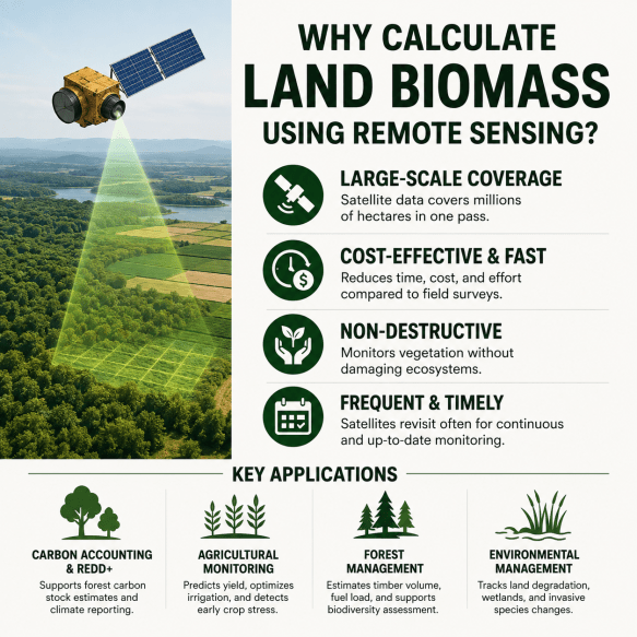
1. Spatial coverage is severely restricted. A field crew can realistically measure biomass across a few dozen plots per season. A satellite covers millions of hectares in a single overpass, making landscape-scale monitoring impossible without remote sensing.

2. Field surveys are expensive and slow. Deploying trained personnel into remote forests or across vast agricultural landscapes requires significant budgets, logistical coordination, and time — all of which scale poorly as survey areas grow.

3. Destructive sampling damages the ecosystem. Harvesting plots to weigh biomass destroys the very vegetation being studied, which is incompatible with long-term monitoring programs that need repeated measurements at the same location.

4. Temporal frequency is too low. Field teams typically survey a site once per year at best. Satellites can revisit the same location every few days, enabling continuous monitoring of seasonal biomass changes and rapid responses to events like fire or drought.

Remote sensing addresses all of these limitations at once. A single Sentinel-2 satellite image covers 290 km² per scene at 10-metre spatial resolution, delivering repeatable, wall-to-wall vegetation data at no marginal cost per additional hectare. The applications that depend on accurate land biomass data are extensive:

• Carbon accounting and REDD+: International climate frameworks require verified estimates of forest carbon stocks. Remote sensing-based biomass maps provide the spatial coverage and update frequency that national forest inventories alone cannot deliver.
• Agricultural monitoring: Crop biomass at different growth stages predicts final yield, informs irrigation scheduling, and flags early stress before it becomes a productivity loss.
• Forest management: Timber volume, fuel load for wildfire risk, and biodiversity assessment all depend on reliable biomass estimates across large forest areas.
• Environmental management: Land degradation monitoring, wetland assessment, and invasive species detection all use biomass change as a primary signal.

How Remote Sensing Measures Land Biomass: The Physical Principles

Every remote sensing system — whether optical satellite, radar, or laser — gathers information about vegetation by measuring how electromagnetic energy interacts with plant material. Understanding this interaction is the key to understanding why remote sensing can estimate biomass at all.

Plants reflect, absorb, and transmit electromagnetic radiation differently depending on their internal chemistry, water content, leaf structure, and canopy architecture. Chlorophyll (the green pigment that powers photosynthesis) strongly absorbs red and blue wavelengths while reflecting green and near-infrared energy.

Healthy, dense vegetation therefore shows a characteristic spectral pattern: low red reflectance, high near-infrared reflectance. This pattern — called the spectral signature — is measurable from space, and its intensity correlates with the amount of plant material per unit area.

From Spectral Signals to Biomass Values

Sensors capture the spectral signature and compute vegetation indices (mathematical ratios that quantify how strongly the vegetation signal appears in a given image). These indices are then linked to biomass through statistical or machine-learning models that are calibrated using field-collected biomass measurements. The result is a spatially continuous biomass map — every pixel in the image gets a predicted biomass value.

The data processing workflow follows a clear sequence. Raw satellite data arrives with geometric distortions and atmospheric interference. Preprocessing corrects these errors. Vegetation indices are calculated from corrected imagery. Field-measured biomass samples serve as the ground truth for model calibration. The validated model is then applied across the full image extent to produce a final biomass map.

Additional physical signals beyond spectral reflectance carry biomass information. Canopy height — how tall the vegetation stands — is a powerful predictor of AGB. Plant density (how many stems per hectare) determines how much light is intercepted. Surface roughness (detected by radar) reflects canopy structural complexity. Sensors that measure these structural properties, rather than just reflectance, often deliver higher biomass estimation accuracy.

Types of Remote Sensing Used for Biomass Estimation

No single sensor dominates biomass estimation across all ecosystems and scales. Scientists and practitioners combine multiple sensor types based on the target vegetation, budget, required accuracy, and geographic coverage.

The most accurate biomass maps today are not built from a single sensor but from the intelligent fusion of optical, radar, and LiDAR data — each filling the blind spots of the others.

1. Optical Satellite Imagery: Multispectral and Hyperspectral

Optical sensors capture reflected sunlight across discrete spectral bands, typically covering visible wavelengths (blue, green, red) and near-infrared (NIR). Multispectral imagery (data from 4–10 spectral bands) forms the backbone of most operational biomass mapping programs worldwide, largely because of the free, continuous data streams from Sentinel-2 and Landsat missions.

Hyperspectral imagery (data from hundreds of narrow, contiguous spectral bands) provides much finer spectral detail. It resolves plant pigments, water content, and leaf chemistry at a level multispectral sensors cannot.

This makes it particularly useful for detecting subtle differences in biomass density across grasslands and agricultural fields. The main limitation of hyperspectral imagery is cloud cover: optical sensors cannot see through clouds, which causes significant data gaps in humid tropical regions where biomass estimation is most critical.

Common satellites used for optical biomass mapping include Landsat 8/9 (30-metre resolution, 16-day revisit), Sentinel-2 (10-metre resolution, 5-day revisit), and PlanetScope (3-metre resolution, daily revisit for commercial applications).

2. Radar (SAR): Seeing Through Clouds and Into Canopies

Synthetic Aperture Radar (SAR) — a system that emits microwave pulses and measures the energy bounced back from the land surface — solves the cloud cover problem entirely. Microwave energy passes through clouds and haze without interference, making SAR the sensor of choice for tropical forest monitoring where persistent cloud cover makes optical imagery nearly unusable.

SAR signals also penetrate into vegetation canopies, interacting with woody stems and branches rather than just the uppermost leaf surface. The longer the radar wavelength, the deeper the signal penetrates. L-band SAR (wavelength around 23 cm, used by ALOS-2 PALSAR-2) penetrates into the lower canopy and interacts with large woody biomass, making it particularly well-suited for tropical forest AGB estimation.

C-band SAR (wavelength around 5 cm, used by Sentinel-1) is more sensitive to surface canopy structure and is widely used for crop biomass monitoring.

Research published in the Journal of Forestry Research (Springer Nature, 2021) found that both L-band ALOS-2 and C-band Sentinel-1 SAR data allowed satisfactory carbon stock estimations, with total carbon stocks in the Mediterranean forest study area reaching approximately 130 t/ha across above-ground, below-ground, deadwood, litter, and soil pools combined.

3. LiDAR: The Gold Standard for Structural Biomass Mapping

LiDAR (Light Detection and Ranging) emits laser pulses and measures the precise time they take to bounce back from the target surface. This timing translates directly into three-dimensional point clouds (dense maps of exactly where each laser pulse reflected) that reveal canopy height, canopy structure, and ground elevation with centimeter-level precision.

Tree height is among the strongest predictors of above-ground biomass — taller trees carry exponentially more biomass than shorter ones. LiDAR-derived height models, combined with field-measured allometric equations (species-specific mathematical relationships between tree height, diameter, and mass), produce biomass estimates that consistently outperform optical or radar approaches in forested landscapes.

NASA’s Global Ecosystem Dynamics Investigation (GEDI) mission — a multi-beam waveform LiDAR instrument mounted on the International Space Station — represents the first purpose-built spaceborne LiDAR system for global biomass estimation. GEDI collects data from 51.6°N to 51.6°S latitude, covering the world’s major tropical and temperate forest zones.

4. Drone-Based Remote Sensing: High-Resolution Field Scale

Unmanned aerial vehicles (UAVs), commonly called drones, bridge the gap between satellite and field-based measurement. A drone carrying RGB cameras captures centimeter-resolution imagery that resolves individual plants.

Multispectral drone sensors compute precise vegetation indices at the plot scale. LiDAR-equipped drones generate dense point clouds that allow biomass estimation with the structural accuracy of airborne LiDAR at a fraction of the cost.

For crop farmers, drone-based biomass mapping is particularly practical. A single flight over a wheat or maize field during the vegetative growth stage produces a biomass density map that flags yield-limiting patches — low-biomass zones that may need supplemental fertilizer or irrigation before the damage becomes irreversible.

Vegetation Indices Used to Estimate Biomass

Vegetation indices are the mathematical bridge between raw spectral reflectance values and biological information about plant density and health. Each index exploits a specific part of the electromagnetic spectrum where vegetation behaves distinctively.

NDVI (Normalized Difference Vegetation Index) is the most widely applied. It divides the difference between near-infrared (NIR) and red reflectance by their sum: NDVI = (NIR – Red) / (NIR + Red). Values range from -1 to +1, with healthy dense vegetation typically scoring between 0.6 and 0.9.

NDVI correlates strongly with Leaf Area Index (LAI — the total one-sided leaf area per unit ground area) and therefore with photosynthetic capacity and biomass accumulation.

• EVI (Enhanced Vegetation Index) corrects for atmospheric effects and soil background interference, making it more reliable than NDVI in high-biomass tropical forests and areas with bright or exposed soil.
• SAVI (Soil-Adjusted Vegetation Index) incorporates a soil brightness correction factor, which is particularly important in arid and semi-arid agricultural settings where bare soil between crop rows strongly influences the spectral signal.
• GNDVI (Green Normalized Difference Vegetation Index) substitutes green reflectance for red in the NDVI formula, making it more sensitive to chlorophyll concentration variations and useful for late-season crop biomass monitoring when canopies are already fully closed.

The Leaf Area Index (LAI) deserves special mention because it is both an output of remote sensing retrieval and a direct driver of biomass accumulation. Plants with higher LAI intercept more solar radiation, fix more carbon, and produce more biomass. Remote sensing-derived LAI maps, generated from MODIS or Sentinel-2 time series, feed directly into crop growth models that simulate yield formation and final harvestable biomass.

Key Data Sources for Land Biomass Estimation

Choosing the right data source depends on the scale of the study, the vegetation type, the required spatial resolution, and the available budget. Below are the primary data streams currently used in operational and research-grade biomass mapping. Free, open-access satellite data from Landsat and the Sentinel constellation has democratized biomass mapping, making it accessible to researchers and agencies that lack the budgets for commercial imagery.

i. Landsat (NASA/USGS): Over 50 years of continuous data, 30-metre resolution, free access. Landsat time series enable historical analysis of biomass change going back to the 1970s, providing unmatched context for deforestation and land degradation monitoring.

ii. Sentinel-2 (ESA): 10-metre resolution in key spectral bands, 5-day revisit, free access. Sentinel-2 is the current standard for crop biomass monitoring and regional forest assessments due to its resolution and frequency combination.

iii. Sentinel-1 (ESA): C-band SAR, all-weather capability, free access. Sentinel-1 is the primary radar source for cloud-affected tropical monitoring and crop biomass in areas where optical data gaps are a persistent problem.

iv. MODIS (NASA): 250m–1km resolution, daily global coverage. MODIS time series are ideal for continental-scale biomass change detection and seasonal monitoring, though the coarse resolution limits utility in fragmented landscapes.

v. PlanetScope: 3-metre resolution, daily revisit, commercial subscription. PlanetScope delivers biomass monitoring at the individual field scale, supporting precision agriculture applications where sub-field spatial variability matters.

vi. NASA GEDI LiDAR: 25-metre footprint diameter, global tropical and temperate coverage, free data products. GEDI is the primary spaceborne source for canopy height and AGB density at the global scale.

vii. ICESat-2 (NASA): Photon-counting LiDAR with global coverage, particularly strong for measuring canopy heights in high-latitude forests and detecting fine-scale height change.

Steps to Calculate Land Biomass Using Remote Sensing

Estimating land biomass using remote sensing data follows a structured workflow. Each step depends on the accuracy of the one before it. Cutting corners in preprocessing or field validation cascades into errors in the final biomass map.

i. Select appropriate imagery: Choose the sensor, spatial resolution, and time period based on your target ecosystem and study objective. Forest biomass monitoring typically requires Sentinel-1 or GEDI data; crop biomass monitoring commonly uses Sentinel-2 or drone multispectral imagery.

ii. Image preprocessing: Apply atmospheric correction to convert raw digital numbers to surface reflectance values. Perform geometric correction to ensure the image aligns accurately with real-world coordinates. Remove cloud-contaminated pixels and replace them using temporal compositing where needed.

iii. Calculate vegetation indices: Compute NDVI, EVI, SAVI, GNDVI, or other relevant indices from the corrected surface reflectance bands. For LiDAR data, derive canopy height metrics (maximum height, 95th percentile height, mean height) from the point cloud.

iv. Collect field biomass samples: Measure above-ground biomass in representative plots within the study area using destructive harvesting or allometric equations applied to tree diameter and height measurements. These field values are the ground truth that anchors the model.

v. Build prediction models: Regress field biomass measurements against the co-located remote sensing variables (vegetation indices, canopy height metrics, SAR backscatter values). Use regression analysis, random forest, support vector machine, or neural network approaches depending on the complexity of the relationship and the amount of training data available.

vi. Validate model results: Use a hold-out validation dataset (field plots not used in model training) to assess prediction accuracy. Report RMSE (Root Mean Squared Error), R² (coefficient of determination), and bias. Refine the model if accuracy is insufficient.

vii. Generate biomass maps: Apply the validated model to the full image extent, producing a spatially continuous biomass density map where each pixel contains a predicted biomass value in Mg/ha or t/ha.

Models and Methods Used for Biomass Estimation

The choice of model significantly influences both the accuracy and the generalizability of a biomass estimation system. Simpler models are more transparent and transfer more reliably to new locations. Complex machine learning models squeeze more accuracy from large training datasets but can overfit to local conditions.

Empirical regression models establish a direct mathematical relationship between field biomass and remote sensing variables — for example, a linear regression between NDVI and crop dry matter yield. These models are easy to interpret and quick to compute, but they perform poorly when the spectral-biomass relationship is non-linear or when biomass values span a very wide range.

Machine learning methods overcome these limitations by learning complex, non-linear relationships from data. Random Forest (an ensemble of decision trees that averages predictions across hundreds of individual trees) is currently the most widely used algorithm for biomass estimation in both forestry and agriculture.

A study published in Frontiers in Plant Science (December 2024) demonstrated that Random Forest applied to GEDI and multi-source remote sensing data produced spruce-fir forest biomass estimates with an R² meaningfully higher than single-sensor regression approaches.

• Support Vector Machine (SVM): Finds the optimal separation boundary between biomass classes in high-dimensional feature space. SVM performs well with small to medium training datasets and is robust against overfitting when properly regularized.
• Neural Networks and Deep Learning: Convolutional Neural Networks (CNNs) and hybrid CNN-LSTM architectures process spatial and temporal patterns in imagery simultaneously. A 2024 study published in Remote Sensing (MDPI) comparing RF, CNN, and CNN-LSTM models for forest biomass estimation in Hangzhou, China found that deep learning models captured spatial context that single-point regression methods missed entirely.
• Hybrid models: Combine physical vegetation models (which simulate plant growth based on radiation and water inputs) with statistical or machine learning calibration layers. These approaches are increasingly favored because they build physically realistic biomass estimates that generalize across regions without relying solely on local training data.

Factors Affecting Biomass Estimation Accuracy

Even the best sensor and model combination produces unreliable biomass maps when the underlying data quality is poor or when the physical environment introduces sources of noise. Understanding these accuracy-limiting factors is essential for anyone designing a biomass mapping program.

1. Dense forest signal saturation: In high-biomass tropical forests, optical and C-band SAR signals saturate — they stop increasing even as biomass continues to rise. NDVI saturates at AGB values above approximately 150–200 Mg/ha, making it unreliable in old-growth tropical forests where biomass may reach 400–600 Mg/ha. L-band SAR and LiDAR saturate at much higher biomass levels and are preferred in these environments.

2. Seasonal variation: Vegetation reflectance changes dramatically across seasons. An NDVI value from a wheat field in April represents a fundamentally different biomass condition than the same field in August. Models must account for seasonal dynamics or be calibrated separately for each phenological stage.

3. Cloud cover interference: Optical sensors lose data wherever clouds are present. In humid tropical regions, cloud contamination can affect more than 70% of image acquisitions in a given year, requiring radar or LiDAR alternatives or multi-year compositing strategies.

4. Mixed pixels: At moderate spatial resolutions (30m–250m), a single image pixel often contains a mixture of crop types, bare soil, and water. The spectral signal reflects the average of all these surfaces, which dilutes the vegetation signal and introduces systematic error into biomass predictions.

5. Terrain effects: Sloped terrain changes the geometry of both solar illumination and sensor viewing angle, altering the reflectance values recorded at the sensor. Topographic correction is mandatory in mountainous areas before any biomass model can be reliably applied.

Applications of Land Biomass Mapping Across Sectors

Land biomass maps generated from remote sensing data feed into practical decision-making across a remarkably wide range of sectors, from government climate reporting to individual farm management.

Forest management agencies use biomass maps to prioritize harvest blocks, estimate sustainable yield, and document compliance with certification standards. Wall-to-wall biomass maps replace expensive sample-based forest inventories in regions where field access is logistically difficult or prohibitively costly.

Carbon stock estimation is one of the most economically significant applications. Every Mg of above-ground biomass contains approximately 0.47 Mg of carbon (the standard IPCC conversion factor). Accurate biomass maps therefore translate directly into verified carbon inventories, which underpin REDD+ payments and voluntary carbon market credits. A verified biomass map covering a 500,000-hectare tropical forest concession can represent hundreds of millions of dollars in carbon assets.

• Precision agriculture: Crop biomass maps derived from drone or Sentinel-2 imagery identify sub-field variability in plant growth, enabling variable-rate fertilizer and irrigation application that reduces input costs while protecting yield.
• Wildfire fuel assessment: Dead wood and dry herbaceous biomass represent the fuel load available to fires. Remote sensing-derived fuel maps guide prescribed burn programs and wildfire containment planning in fire-prone landscapes.
• Biodiversity conservation: High-biomass, structurally complex vegetation typically supports greater species diversity. Biomass maps help identify priority conservation areas and track the recovery of restored habitats over time.
• Bioenergy planning: Governments and energy companies use remote sensing biomass data to assess the sustainable supply of agricultural residues and woody biomass for bioenergy production, ensuring that harvest rates do not exceed ecosystem regeneration capacity.

Advantages of Remote Sensing for Biomass Calculation

Remote sensing-based biomass mapping offers a combination of capabilities that no ground-based approach can match. These advantages explain why the technology has moved from experimental to operational status across dozens of countries in the past decade.

Non-destructive measurement is perhaps the most fundamental advantage. Remote sensing gathers information about vegetation without harvesting, cutting, or disturbing it. This enables repeated measurements at exactly the same location, which is essential for detecting biomass change over time — the metric that matters most for carbon accounting and ecosystem monitoring.

• Large-scale coverage at low marginal cost: Once the sensor and processing pipeline are set up, the cost of adding another million hectares to a biomass survey is essentially zero. This cost structure is the inverse of field surveys, where costs scale linearly with area.
• Frequent temporal updates: Sentinel-2 revisits any location on Earth every 5 days. This frequency allows biomass monitoring across the entire growing season, capturing dynamic changes that single annual field surveys completely miss.
• Historical analysis capability: The Landsat archive contains imagery from 1972 onward. Researchers can reconstruct historical biomass trajectories to quantify cumulative deforestation, assess ecosystem recovery after disturbance, or establish pre-disturbance baseline conditions for compensation claims.
• Improved decision-making for land managers: Spatially explicit biomass maps reveal where within a landscape biomass is accumulating, declining, or stable — giving land managers the spatial precision to target interventions where they will have the greatest impact.

Limitations and Challenges in Remote Sensing Biomass Estimation

Remote sensing biomass mapping is powerful, but it comes with real technical limitations that practitioners must understand before relying on the outputs for high-stakes decisions.

Signal saturation in dense forests remains an unresolved challenge for optical and C-band radar sensors. As tree canopy closes and biomass accumulates beyond a sensor-specific threshold, the spectral or backscatter signal no longer increases with biomass.

LiDAR avoids this problem because it measures physical structure rather than spectral reflectance, but airborne LiDAR data collection remains expensive, and spaceborne LiDAR like GEDI provides sparse, non-contiguous footprints rather than wall-to-wall coverage.

• Field validation is mandatory: No remote sensing model produces reliable biomass estimates without calibration and validation against actual field measurements. The quality of the field data directly determines the quality of the final map — and collecting representative field data in heterogeneous landscapes is both expensive and technically demanding.
• Atmospheric effects require careful correction: Aerosols, water vapor, and ozone scatter and absorb incoming and reflected solar radiation, altering the spectral signal before it reaches the sensor. Incorrect or incomplete atmospheric correction introduces systematic errors that propagate through the entire biomass estimation workflow.
• Data processing requires specialized expertise: Working with remote sensing time series at scale requires knowledge of geographic information systems (GIS), programming languages like Python or R, and cloud-based geospatial platforms like Google Earth Engine. This technical barrier limits adoption among agronomists and land managers without data science backgrounds.
• Model uncertainty grows with distance from training data: A biomass model calibrated in a Brazilian Amazon forest may perform poorly when transferred to a structurally different West African forest, even if both are classified as tropical moist forest. Regional calibration datasets are essential for maintaining accuracy across geographically diverse study areas.

Future Trends in Remote Sensing Biomass Estimation

The technology landscape for land biomass mapping is evolving rapidly. Several converging trends are set to substantially improve the accuracy, accessibility, and operational scalability of biomass estimation over the next five to ten years.

AI-powered biomass mapping represents the most transformative development underway. Deep learning architectures — particularly convolutional and transformer-based models — process the full spectral, spatial, and temporal information in satellite time series simultaneously, extracting biomass signals that simpler models cannot detect.

AI and machine learning integration in remote sensing grew by 35% between 2021 and 2026, according to Business Research Insights, fundamentally reshaping how vegetation data is analyzed at scale.

The European Space Agency’s BIOMASS mission, launched in 2024, carries the first spaceborne P-band SAR specifically designed for tropical forest biomass monitoring. P-band signals (wavelength around 70 cm) penetrate deep into forest canopies, reaching woody stems and large branches that shorter-wavelength radars cannot access.

Research published in Scientific Reports (April 2023) demonstrated that P-band TomoSAR (Tomographic SAR — a technique that reconstructs three-dimensional forest structure from multiple radar passes) produced promising AGB estimates across dense tropical forests in French Guiana, providing a preview of what the BIOMASS mission will deliver operationally.

• Multi-sensor data fusion at scale: Algorithms that automatically combine optical, radar, and LiDAR data streams — weighting each sensor according to its reliability in a given ecosystem and season — are moving from experimental prototypes toward operational tools deployed on cloud platforms.
• Real-time and near-real-time biomass monitoring: Cloud-based geospatial platforms like Google Earth Engine and Microsoft Planetary Computer now enable continuous, automated processing of incoming satellite data streams. Near-real-time deforestation alerts that trigger within 24–48 hours of forest loss events are already operational in several tropical countries.
• Digital twins for precision agriculture: Integrating remote sensing-derived biomass data with soil sensors, weather models, and crop simulation models creates farm-scale digital twins — virtual replicas of real fields that allow farmers to test management scenarios before implementing them in the real world.
• Precision agriculture integration: The convergence of affordable drone sensors, satellite time series, and AI-driven analytics is making field-scale biomass monitoring financially accessible to individual farmers for the first time, not just to research institutions and government agencies.

1. Which satellite is best for biomass estimation? There is no single best satellite for all situations. Sentinel-2 is the most widely used for crop and moderate-resolution forest biomass mapping. GEDI LiDAR provides the most accurate canopy height data for forest AGB. Sentinel-1 SAR is the preferred choice in cloud-affected tropical areas. The best operational approach combines multiple sensors.

2. Can drones estimate biomass accurately? Yes. Drones equipped with multispectral cameras or LiDAR sensors can estimate crop and small-area forest biomass with very high spatial resolution. Drone-based biomass estimates for crops typically achieve correlations of R² = 0.80–0.95 with field measurements when flights are timed to appropriate growth stages and spectral sensors are properly calibrated.

3. How accurate is remote sensing biomass estimation? Accuracy varies considerably by sensor type, ecosystem, and model approach. In temperate forests with good LiDAR coverage, biomass maps can achieve RMSE values of 20–40 Mg/ha. In dense tropical forests, optical-only approaches may show RMSE values of 60–100 Mg/ha due to signal saturation. Multi-sensor fusion models consistently outperform single-sensor approaches.

4. Why is biomass estimation important for climate change? Forests and agricultural landscapes store massive amounts of carbon in their biomass. Deforestation and land degradation release this stored carbon as CO₂ into the atmosphere, accelerating climate change. Accurate biomass maps provide the foundation for verifying carbon stocks, monitoring forest loss, and quantifying the effectiveness of reforestation and conservation programs under international climate frameworks like REDD+.

5. Can remote sensing estimate below-ground biomass? Remote sensing cannot directly measure below-ground biomass. However, BGB is commonly estimated from AGB using root-to-shoot ratio coefficients derived from field studies and published by organizations like the IPCC. Species-specific root-to-shoot ratios range from 0.15 to 0.40 in most forest ecosystems, allowing indirect BGB estimation wherever AGB maps exist.

Conclusion

Land biomass calculated using remote sensing has moved decisively from a specialized research technique to an operational capability with direct implications for food production, forest governance, and climate policy. The convergence of free satellite data, accessible cloud computing platforms, and increasingly powerful machine learning tools has made landscape-scale biomass mapping achievable for a growing number of organizations worldwide.

The role of remote sensing in climate monitoring will only grow as carbon markets expand, deforestation monitoring commitments intensify, and the demand for verified carbon stock data escalates across the global economy. With the BIOMASS satellite mission now operational, GEDI continuing to extend its global dataset, and AI models dramatically improving estimation accuracy from multi-sensor data fusion, the ability to know precisely where biomass is accumulating, declining, or remaining stable across the Earth’s land surface is within reach.

Carbon markets have moved from niche policy experiments to mainstream climate finance instruments. The voluntary agriculture carbon credit market was valued at USD 36.1 million in 2024 and is expected to surge to USD 648.3 million by 2034 at a 31.9% CAGR, according to Global Market Insights Inc. Agriculture sits at the center of this expansion because soils, crops, and land management practices represent enormous, measurable carbon sinks.

The challenge has always been measurement: how do you reliably quantify carbon stored across millions of hectares of farmland? Remote sensing, the science of collecting data about the Earth’s surface from aircraft, drones, and satellites without physical contact, is the answer the carbon market has been waiting for. It brings scale, speed, and scientific rigor to agricultural carbon monitoring.

What Are Carbon Credits and Why Do They Matter?

A carbon credit is a tradable certificate representing the reduction or removal of one metric ton of carbon dioxide equivalent (CO2e) from the atmosphere. Credits come in two types: carbon reduction credits, which represent emissions avoided, and carbon removal credits, which represent CO2 actively pulled from the atmosphere and stored.

Carbon markets function as economic mechanisms that put a price on greenhouse gas emissions. When a company cannot reduce its emissions internally, it can purchase carbon credits from projects that remove or avoid an equivalent quantity.

This creates financial incentives for activities like soil carbon sequestration, reforestation, and improved land management. The system is governed by carbon registries, certification standards, and third-party verifiers who ensure each credit represents a real, measurable climate benefit.

1. How Carbon Credits Are Generated in Agriculture

Agricultural carbon credits are created through a structured process that begins with project design and ends with verified credits listed on a registry. Here is the typical sequence:

1. A farmer or project developer selects eligible sustainable farming practices and defines the project boundary.
2. An approved methodology is chosen from a carbon registry such as Verra (VM0042) or Gold Standard.
3. A baseline carbon stock is established to measure the starting point before practices change.
4. Practices are implemented and monitored across the project period, typically three to five years.
5. Independent third-party verifiers assess whether practices were implemented and whether claimed carbon benefits are real and additional.
6. Verified carbon credits are issued and listed for sale on voluntary or compliance markets.

Soil carbon sequestration through conservation practices is the primary mechanism in cropland projects. Practices such as cover cropping, reduced tillage, and precision nutrient management increase the amount of organic carbon stored in agricultural soils, which otherwise tend to lose carbon through tillage and erosion.

Agricultural soils hold roughly three times more carbon than the atmosphere. This makes farmland one of the most accessible and scalable carbon sinks on the planet. Croplands and grasslands respond quickly to management changes: switching from conventional tillage to zero-tillage can begin increasing soil organic carbon within one to two growing seasons.

Farmers benefit directly from carbon credit revenue. Soil carbon projects now account for approximately 8-10% of the voluntary carbon market, valued at USD 425-530 million, according to 2025 market data.

That revenue stream supplements farm income while simultaneously improving soil health, water retention, and long-term productivity. Agribusinesses and food companies participating in carbon programs also gain credibility in supply chain sustainability reporting.

Connection Between Carbon Credits and Precision Agriculture

Precision agriculture is a farm management approach that uses spatial data and advanced technology to make decisions at the sub-field level rather than treating an entire farm as a uniform unit. It combines GPS (Global Positioning System) receivers, IoT (Internet of Things) soil sensors, drone-mounted cameras, and satellite imagery to deliver detailed, location-specific information about crop conditions, soil properties, and resource needs.

The result is data-driven farm management. Instead of applying a blanket rate of fertilizer across an entire field, a precision agriculture system identifies zones with different nutrient needs and applies variable rates accordingly.

This reduces input waste, lowers operating costs, and produces measurable environmental benefits that can be quantified for carbon credit programs. Precision tools contribute to carbon outcomes through multiple pathways.

• Optimizing fertilizer application reduces nitrous oxide (N2O) emissions, a greenhouse gas roughly 273 times more potent than CO2 over a 100-year period. Variable-rate nitrogen application can cut N2O emissions by up to 20-30% compared to uniform application, according to research published in the European Journal of Agronomy.
• Improving irrigation scheduling with soil moisture sensors reduces energy consumption at pumping stations and limits soil compaction, both of which reduce the carbon footprint of irrigation.
• Maintaining soil health through reduced tillage preserves soil aggregate structure, protecting the organic matter that holds carbon in place over the long term.
• Reducing fuel use through GPS-guided machinery path planning lowers diesel consumption, directly reducing CO2 emissions from field operations.

1. Sustainable Farming Practices That Generate Carbon Credits

Not all farming activities qualify for carbon credits. Approved practices must demonstrably increase soil carbon, reduce emissions, or both. The following practices have established methodologies under major carbon registries.

i. Cover Cropping involves planting non-cash crops during the off-season to keep living roots in the soil. Roots continuously secrete sugars that feed soil microbes, which convert organic matter into stable humus, a long-lived form of soil carbon. Cover crops also prevent erosion, which physically removes topsoil and the carbon within it.

ii. Zero-Tillage and Reduced Tillage minimize soil disturbance, preserving the physical structure of the soil. Conventional tillage oxidizes soil carbon rapidly by exposing organic matter to air. Research published in the journal Soil and Tillage Research has shown that long-term no-till adoption increases soil organic carbon concentration in the top 30 cm by an average of 10-30% compared to conventional tillage over a ten-year period.

iii. Crop Residue Retention keeps post-harvest biomass on the field surface rather than burning or removing it. As residue decomposes, it contributes organic matter to the soil and feeds the microbial communities responsible for carbon fixation. Satellite imagery can measure residue cover percentages after harvest with measurable accuracy.

Remote sensing does not just observe agriculture from above. It transforms scattered field-level data into a unified, scientifically defensible record of how land is managed and how much carbon it holds.

iv. Precision Nutrient Management uses variable-rate technology to apply fertilizers where needed, in the right quantities, at the right time. This reduces the pool of excess nitrogen that soil bacteria convert to nitrous oxide, directly cutting the greenhouse gas footprint of crop production.

v. Agroforestry and Perennial Crops sequester carbon both above ground in woody biomass and below ground through extensive, long-lived root systems. Tree crops can store carbon for decades, making them high-value candidates for carbon credit projects that require permanence.

Role of Remote Sensing in Carbon Credit Measurement

Carbon credit programs require evidence. Registries cannot accept a farmer’s self-reported claim that cover crops were planted or that tillage was reduced. Verification demands objective, reproducible, and auditable data, preferably from sources that cannot be manipulated after the fact. Remote sensing provides exactly this.

Satellite and drone-based observations cover vast areas simultaneously, offering a level of spatial coverage that field surveys simply cannot match economically. The agriculture carbon MRV satellite market was valued at USD 3.2 billion in 2025 and is projected to reach USD 8.7 billion by 2034 at a 12.8% CAGR, signaling how central satellite-based monitoring has become to climate programs globally.

Sustainability Atlas (2026) found that satellite-based verification systems reduced soil carbon measurement costs by 40% compared to traditional field sampling, with investment in digital MRV solutions reaching USD 2.3 billion in 2025. Farmers and project developers can now access credible carbon monitoring without the prohibitive per-hectare cost of repeated soil sampling campaigns.

1. Remote Sensing Technologies Used in Carbon Programs

Several sensor types are deployed depending on the scale, crop type, and carbon measurement objective. Each brings distinct advantages.

1. Multispectral Sensors capture reflected light in discrete wavelength bands, including visible red, near-infrared, and shortwave-infrared. They calculate vegetation indices such as NDVI (Normalized Difference Vegetation Index), a ratio that compares near-infrared reflectance to red reflectance.

Healthy, dense vegetation reflects more near-infrared and absorbs more red light, producing a high NDVI value. NDVI is widely used as a proxy for biomass density and photosynthetic activity, both of which correlate with carbon uptake.

2. Hyperspectral Sensors capture hundreds of narrow, contiguous wavelength bands instead of a handful of broad ones. This finer spectral resolution allows them to detect subtle differences in plant biochemistry, including chlorophyll content, leaf water, and lignin concentration.

These properties are closely linked to above-ground carbon content and can be used to model crop biomass with greater precision than broadband multispectral data.

3. LiDAR (Light Detection and Ranging) fires thousands of laser pulses per second at the ground surface and measures the time it takes for each pulse to return. The result is a detailed three-dimensional point cloud of the landscape, capturing vegetation height, canopy density, and terrain topography.

Biomass is estimated by combining these structural measurements with allometric equations, mathematical relationships that convert height and volume into dry mass and carbon content. A 2025 study in ScienceDirect found LiDAR-based carbon sequestration measurement achieved significantly lower error rates than conventional field inventory methods for forested croplands and agroforestry systems.

4. SAR (Synthetic Aperture Radar) transmits microwave energy and measures the energy reflected back from the surface. Unlike optical sensors, SAR penetrates cloud cover and operates at night, making it valuable in tropical agricultural regions where persistent cloud cover blocks optical satellites for weeks at a time. SAR is particularly effective for measuring soil moisture, detecting bare versus vegetated surfaces, and estimating canopy biomass through backscatter intensity analysis.

5. Drone-Based Remote Sensing delivers centimeter-level spatial resolution that satellites cannot match. Drones equipped with multispectral or RGB cameras fly at low altitude to produce extremely detailed maps of individual fields.

In carbon programs, drones are used for local-scale validation of satellite observations and for assessments in small or fragmented fields where satellite pixel size is too coarse to distinguish management boundaries. The major satellite platforms supporting carbon monitoring include the following:

• Landsat (NASA/USGS): 30-meter resolution with a 16-day revisit frequency. Its historical archive dating back to 1972 makes it the backbone of long-term land use change analysis and baseline mapping.
• Sentinel-1 and Sentinel-2 (ESA): Sentinel-2 provides 10-meter multispectral imagery with a 5-day revisit, making it ideal for seasonal crop monitoring. Sentinel-1 SAR complements optical data during cloudy periods.
• MODIS (NASA): 250-500 meter resolution with daily global coverage. It is used for large-scale, time-series analysis of vegetation productivity and land use change across entire regions.
• PlanetScope: A commercial constellation delivering 3-meter resolution daily imagery, enabling sub-field practice detection across individual farm operations.

How GeoPard Supports Carbon Credit Programs

GeoPard Agriculture is a precision agriculture platform that combines satellite imagery, radar data, and topography analytics to help farmers implement and monitor the practices that generate verified carbon credits. It integrates carbon farming directly into everyday farm management rather than treating it as a separate activity.

1. Practice Implementation Guided by Satellite Data

GeoPard uses satellite and radar data to identify low-performing field zones suitable for cover cropping, agroforestry, or tillage reduction. Its crop monitoring solution guides rotation decisions that improve soil structure and increase long-term carbon storage capacity.

Topography analytics pinpoints which field areas benefit most from specific cover crop species, removing guesswork from a practice that directly drives carbon sequestration.

2. Emission Reduction and MRV Traceability

For CO2 reduction, GeoPard supports zero-tillage adoption and residue management by helping farmers transition away from conventional soil disturbance. For N2O reduction, it enables 4R nutrient management, applying the right fertilizer, at the right rate, time, and place, cutting the excess nitrogen that converts to nitrous oxide in the soil.

On the MRV side, GeoPard’s satellite data layers create a continuous, time-stamped record of field activities throughout the growing season. This spatial evidence supports measurement and reporting requirements, giving third-party verifiers objective data to confirm that claimed practices actually happened.

By connecting daily farm decisions directly to measurable carbon outcomes, GeoPard makes it practical for farmers of all scales to participate in carbon credit programs with confidence.

How Remote Sensing Enables Carbon Credits: Step-by-Step

1. Baseline Mapping

Before a carbon project can issue any credits, it must establish a credible baseline, a quantified snapshot of how much carbon the project area already holds and what land management practices are currently in place. This baseline is the reference against which all future improvements are measured.

Remote sensing enables baseline mapping through several integrated analyses. Vegetation mapping using NDVI and leaf area index data identifies existing crop types, biomass density, and growing season patterns.

Historical land-use analysis using Landsat’s multi-decade archive reveals whether a field has been under conventional tillage, grassland, or mixed cropping for the past ten to twenty years. This history matters because soil carbon levels reflect cumulative management over decades, not just the current season.

Soil property mapping combines hyperspectral satellite data with ground-truth soil samples to produce spatially continuous maps of soil organic carbon, texture, and clay content. Project boundary identification uses GPS-registered satellite imagery to define the exact geographic limits of the carbon project, a requirement for all major carbon registries including Verra and Gold Standard.

2. Practice Verification

Carbon registries require ongoing evidence that sustainable practices are genuinely implemented, not just claimed. Remote sensing provides this evidence through time-series analysis of satellite imagery across entire growing seasons.

i. Cover Crop Detection uses winter-season vegetation indices to identify actively growing ground cover between cash crop cycles. A field with cover crops shows significantly higher NDVI values during the off-season compared to a bare field.

Research published in the National Center for Biotechnology Information (2024) using Sentinel-2 data in South Dakota achieved classification accuracies exceeding 80% for detecting the presence of cover crops and tillage intensity across corn and soybean fields.

A ScienceDirect study (2024) deployed an MRV pipeline across 553,743 hectares and measured emission reductions of 398,408.5 tCO2e across three consecutive carbon credit issuances, attributing reductions primarily to cover crop introduction and tillage intensity reduction. Satellite-based MRV systems can now operate at the scale of entire farming regions, not just individual project sites.

ii. Zero-Tillage Verification relies on monitoring the soil surface between harvest and planting. After a no-till harvest, residue remains on the surface and NDVI values remain moderately elevated due to residue reflectance. A tilled field shows abrupt changes in surface texture and spectral signature that are detectable in 10-30 meter satellite imagery. SAR data supplements optical analysis by detecting soil moisture changes associated with mechanical disturbance.

iii. Crop Residue Retention Monitoring uses shortwave-infrared bands to estimate the percentage of crop residue covering the soil after harvest. Residue has a distinct spectral signature compared to bare soil, allowing satellite-derived residue cover indices to estimate whether 30%, 50%, or 70% of the surface is covered, thresholds that directly determine eligibility and credit volume in many methodologies.

iv. Crop Rotation Monitoring tracks changes in crop type across multiple seasons using spectral time-series data. Different crops have unique phenological fingerprints, the pattern of greenup, peak growth, and senescence over the growing season. Sentinel-2’s 5-day revisit frequency captures these dynamics precisely enough to distinguish maize from soybeans from wheat across consecutive years.

3. Biomass and Carbon Stock Estimation

Measuring carbon stocks requires converting observable vegetation and soil properties into quantitative estimates of stored carbon. Remote sensing feeds this process through multiple data streams.

Above-Ground Biomass (AGB) estimation uses vegetation height from LiDAR data, canopy density from optical imagery, and Leaf Area Index (LAI) derived from near-infrared reflectance. These inputs feed allometric equations that produce biomass estimates in tons per hectare. Carbon content is typically calculated as approximately 47-50% of dry biomass weight, a conversion factor validated across hundreds of species by the IPCC and FAO.

Soil Organic Carbon (SOC) estimation is more complex because below-ground carbon cannot be directly observed from above. Remote sensing contributes through hyperspectral imagery that detects soil organic matter spectral signatures in bare or lightly vegetated fields, and through SAR-derived soil moisture data that influences carbon turnover rates.

These remote sensing inputs are combined with process-based models like RothC or CENTURY, which simulate how organic matter decomposes and stabilizes under different climate and management conditions.

The credibility of a carbon credit depends entirely on the precision of the measurement behind it. Remote sensing shifts carbon verification from an expensive field exercise into a continuous, data-driven audit trail.

Machine learning algorithms, including random forests, gradient boosting, and deep learning models, are increasingly used to integrate remote sensing inputs with field measurements.

Research published in PeerJ (2024) demonstrated that machine learning models combining multispectral satellite indices with limited soil sampling could predict soil organic carbon with competitive accuracy, reducing the number of destructive soil samples required for project validation.

Measurement, Reporting, and Verification (MRV): Foundation of Carbon Credits

MRV (Measurement, Reporting, and Verification) is the governance framework that separates credible carbon credits from unverifiable claims. Every major carbon registry requires projects to follow an approved MRV protocol. Remote sensing has become an integral part of all three stages.

1. Measurement: Collecting the Data

Measurement involves collecting the raw data from which carbon quantities are calculated. In satellite-based programs, this begins with automated ingestion of multispectral and SAR imagery at regular intervals throughout the growing season.

Drone surveys provide high-resolution ground data at key phenological stages. Targeted soil sampling campaigns collect in-field measurements to calibrate and validate satellite-derived SOC estimates. Biomass estimation algorithms run on the combined data to produce field-scale carbon stock values.

2. Reporting: Converting Measurements into Credits

Reporting transforms processed data into a formal documentation package submitted to a carbon registry. This includes carbon accounting spreadsheets, spatial maps of project activities, evidence of practice implementation, and modeled carbon stock changes over the verification period.

Compliance with international standards, including ISO 14064-2 and GHG Protocol guidelines, is required. Satellite time-series archives serve as tamper-proof records that underpin every reported figure.

3. Verification: Independent Confirmation

Third-party verifiers review the submitted documentation and independently assess whether the reported carbon outcomes are real, additional (meaning they would not have occurred without the project), and permanent.

Remote sensing evidence, including satellite image archives and drone surveys, provides verifiers with objective data to compare against project claims. Time-series analysis detects inconsistencies, such as a farmer claiming zero-tillage for a field that shows spectral signatures of mechanical disturbance.

Fraud detection through change-point algorithms is increasingly embedded in digital MRV platforms to flag anomalies before they reach the verification stage.

According to data reported by Marq Stats (2026), the convergence of high-resolution satellite imagery and machine learning reduced the cost of per-farm MRV by 70-90% between 2018 and 2025, enabling Indigo Carbon to manage over 8 million enrolled acres across 28 U.S. states with an 85% reduction in administrative data collection burden.

Cost reductions at this scale mean that smallholder farmers and mid-sized operations can now participate in carbon credit programs that were previously only accessible to large commodity producers.

4. How MRV Determines the Real Value of a Carbon Credit

MRV is not just a compliance requirement. It is what determines whether a carbon credit has real market value or not. Buyers, investors, and regulators all price carbon credits based on how confidently the underlying carbon can be verified. A credit with weak MRV trades at a discount or gets rejected entirely.

Without credible MRV, carbon credits become guesswork. A farmer could claim cover crops were planted when they were not. A project developer could overestimate soil carbon gains. Buyers could unknowingly fund projects that deliver no real climate benefit. MRV closes each of these gaps by requiring documented, verifiable, and standardized evidence at every step.

For farmers, strong MRV works in their favor. It removes the burden of self-reporting and replaces it with satellite-backed evidence that no registry or buyer can dispute. That shift from trust-based to data-based verification is what allows smallholder farmers to compete in the same carbon markets as large agribusinesses.

For the carbon market as a whole, credible MRV is what separates genuine climate action from greenwashing. Every ton of CO2 that gets counted twice, estimated loosely, or claimed without evidence weakens the entire system.

Remote sensing-powered MRV closes that gap by making the measurement objective, the reporting standardized, and the verification independent. This is why carbon credits backed by satellite-based MRV now command a 15-25% price premium in voluntary markets — buyers pay more because the science behind the credit is harder to dispute.

Benefits of Remote Sensing for Carbon Credit Programs

The advantages of remote sensing over purely field-based carbon monitoring are substantial and compound as programs scale to cover more land.

1. Large-scale monitoring becomes feasible at a fraction of the cost. A single Sentinel-2 scene covers 100 by 100 kilometers, monitoring thousands of farms in a single pass without any ground crew involvement.
2. Verification is faster and less labor-intensive. Carbon programs that previously required months of field visits can complete practice verification within days using automated satellite analysis pipelines.
3. Transparency increases for buyers, registries, and investors. Satellite archives create an objective, reproducible record of what happened on a field during the project period, independent of any stakeholder’s interest.
4. Human error is reduced. Automated image classification and carbon modeling apply consistent algorithms across all project areas, eliminating variation introduced by different field assessors using different sampling methods.
5. Investor confidence grows. Institutional buyers increasingly require quantitative, data-backed credit validation before committing capital to carbon projects. Remote sensing-backed credits with Core Carbon Principles (CCP) labels now command 15-25% price premiums, according to the Integrity Council for the Voluntary Carbon Market’s 2025 data.

Better decision-making flows to every stakeholder. Farmers receive spatially explicit feedback about which fields are performing well or underperforming for carbon outcomes. Project developers can allocate monitoring resources to high-risk zones. Registries can prioritize verification efforts based on automated anomaly detection.

Challenges and Limitations in Carbon Markets

Remote sensing is powerful but not unlimited. Understanding its current constraints is essential for designing carbon programs that remain scientifically defensible.

1. Cloud cover remains a persistent obstacle for optical satellite sensors in tropical and monsoon-affected agricultural regions. During key periods of the growing season, consecutive cloud-free observations may be impossible, creating gaps in the monitoring record. SAR partially compensates for this, but integrating multi-sensor datasets adds processing complexity.
2. Below-ground carbon cannot be directly observed from space. Soil organic carbon estimation through remote sensing is always model-dependent, relying on surface spectral proxies and process-based simulations that carry inherent uncertainty.
3. Spatial resolution limits practice detection at small field scales. In regions dominated by smallholder agriculture with fields smaller than one hectare, even 10-meter Sentinel-2 pixels may straddle multiple management boundaries, making clean practice attribution difficult.
4. Ground-truth validation remains mandatory. Satellite models require calibration with in-field soil samples and field observations. No current remote sensing methodology eliminates the need for ground data entirely.

Standardization across carbon programs is another challenge. Different registries accept different remote sensing methodologies, different satellite platforms, and different modeling approaches. A credit validated using one methodology may not be recognized by a buyer operating under a different standard, creating market fragmentation that limits credit liquidity and farmer participation.

Future of Remote Sensing in Carbon Markets

The pace of innovation in satellite technology, artificial intelligence, and digital agriculture infrastructure suggests that the limitations of today’s remote sensing systems will be progressively resolved over the next decade.

Artificial intelligence and machine learning are already transforming carbon estimation. Deep learning models trained on millions of satellite pixels can identify tillage patterns, crop types, and practice changes with greater accuracy and at lower per-field cost than any previous method.

Frontier models published in Remote Sensing of Environment (2024) demonstrated that hyperspectral machine learning models could predict soil organic carbon across continental scales with competitive accuracy when trained on spatially diverse soil spectral libraries.

High-resolution commercial satellite constellations, including PlanetScope’s 3-meter daily coverage and upcoming very high-resolution systems, are making sub-field practice monitoring accessible to programs operating at individual farm level.

Drone and satellite data fusion is enabling a layered monitoring approach: satellites provide continuous coverage while drones provide validation detail when and where it is needed most.

• IoT integration allows real-time soil sensor data from networks of in-field moisture and carbon probes to feed directly into remote sensing calibration pipelines, reducing reliance on periodic manual soil sampling.
• Digital twins for agricultural landscapes are emerging as a way to simulate carbon dynamics across an entire farm using combined remote sensing, weather, and soil data inputs. These simulation environments allow project developers to model “what-if” scenarios for different practice combinations before committing to a methodology.
• Blockchain-enabled carbon tracking links satellite-verified carbon events to immutable ledger records, providing buyers with a complete audit trail from field observation to credit retirement.
• Automated MRV platforms are replacing manual data submission workflows. Companies like Agreena in Denmark are using earth observation data to monitor land management changes across thousands of farms in the EU, with carbon credits issued based on continuous satellite analysis under the EU’s Carbon Farming Regulation (EU 2024/3012).

Near real-time carbon monitoring, with satellite revisit frequencies approaching daily and analysis pipelines that process imagery within hours of acquisition, will soon make it possible to detect practice reversals, such as a farmer returning to tillage mid-project, before significant carbon loss occurs. Global satellite constellations and expanding processing infrastructure are bringing this capability within reach for major carbon registries by the late 2020s.

Conclusion

How remote sensing enables carbon credits comes down to one core advantage: it turns the invisible into the measurable. Carbon stored in soils and vegetation cannot be directly weighed or counted. But the farming practices that determine how much carbon a landscape holds, including what is planted, how the soil is managed, and how biomass is distributed, all leave detectable spectral and structural signatures that satellites, LiDAR systems, and SAR platforms can observe, record, and quantify.

From baseline mapping to practice verification, from biomass estimation to MRV documentation, remote sensing provides the scientific foundation that carbon markets require to function with integrity. The connection between precision agriculture and carbon markets has never been stronger. Farmers who adopt data-driven management practices are not only improving their productivity. They are generating the kind of verifiable, spatially explicit carbon evidence that registries, buyers, and regulators increasingly demand.

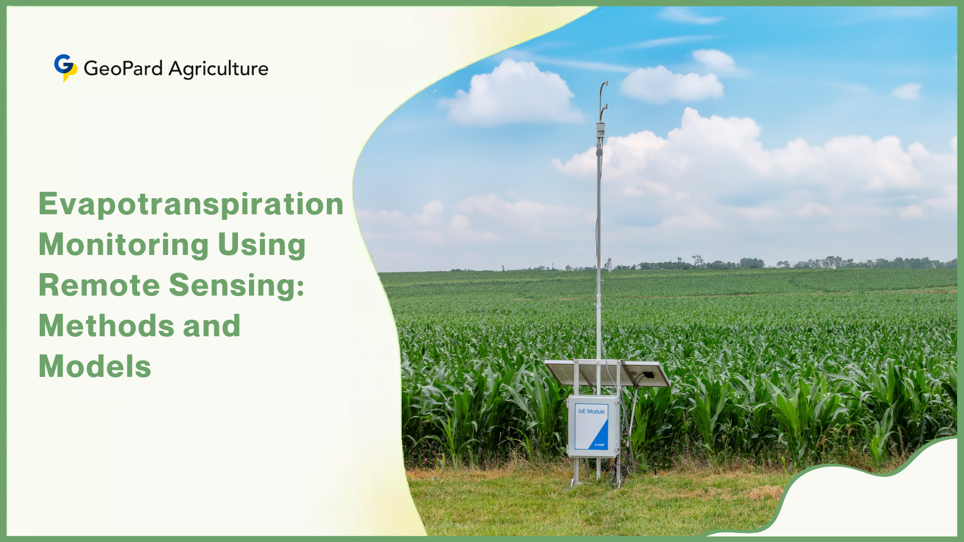
Evapotranspiration monitoring with remote sensing represents one of the most consequential advances in agricultural water science of the past two decades. By combining satellite-derived thermal data, vegetation indices, and energy balance physics, scientists and farmers can now estimate how much water leaves the land surface across millions of hectares — without a single ground-based sensor.

This capability is transforming how agronomists schedule irrigation, how governments track drought, and how researchers quantify the water footprint of entire river basins. Agriculture consumes roughly 70% of all global freshwater withdrawals, yet most of this water is never directly measured at the field level — a critical gap that evapotranspiration monitoring with remote sensing is rapidly closing.

What Is Evapotranspiration?

Evapotranspiration (ET) is the combined process through which water moves from the land surface into the atmosphere. It has two components working simultaneously: evaporation, the direct conversion of liquid water from soil, water bodies, and plant surfaces into water vapor; and transpiration, the biological movement of water absorbed by plant roots, transported upward through the stem, and released as vapor through tiny pores in leaves called stomata.

Together, these two processes account for the largest flux of water leaving a terrestrial ecosystem. In most agricultural landscapes, ET returns between 60 and 80 percent of all precipitation back to the atmosphere. That figure makes ET the dominant variable in the land water balance — more influential than runoff or deep percolation in most cropped environments.

ET sits at the center of the hydrological cycle, linking the land surface, the biosphere, and the atmosphere. When ET rates are high, soil moisture depletes faster, river baseflows decline, and aquifer recharge rates drop. When ET slows — due to drought stress, crop senescence, or land-use change — the consequences ripple through water availability downstream.

In climate science, ET is a primary coupling mechanism between the carbon and water cycles. Plants open their stomata to absorb CO2 for photosynthesis, and in doing so, they simultaneously release water vapor. Any change in global vegetation cover, temperature, or CO2 concentration shifts the planetary ET balance and feeds back into regional precipitation patterns.

Why Monitoring Evapotranspiration Is a Water Management Priority?

Precise ET data drives better decisions across multiple sectors. In agriculture, knowing actual crop water use at the field level tells an irrigation manager exactly how much water to apply, when to apply it, and where deficits are developing before visible stress appears in the crop.

This precision prevents both over-irrigation, which wastes water and leaches nutrients, and under-irrigation, which suppresses yield.

1. Irrigation scheduling: ET-based irrigation scheduling replaces guesswork with physics. When a farmer knows that a corn field in July is losing 7 mm of water per day to ET, they can replenish that exact deficit rather than irrigating on a fixed calendar interval.

2. Drought monitoring: A sustained drop in actual ET relative to the reference ET (what would evaporate under unlimited water supply) signals emerging drought stress. Remote sensing captures this signal weeks before yield loss becomes visible to the eye.

3. Water resource planning: Basin-level water accounting requires ET data at the watershed scale. Satellite ET monitoring provides this spatial coverage at a fraction of the cost of a ground station network.

4. Climate change assessment: Long-term ET trends reveal how warming temperatures and shifting precipitation patterns are altering ecosystem water use — data that informs adaptation planning at the regional and national level.

5. Ecosystem health monitoring: Wetland ET rates, forest transpiration, and grassland water use all respond sensitively to ecological disturbance. Remote sensing ET catches these changes across large, inaccessible landscapes.

What Factors Influence Evapotranspiration?

Evapotranspiration (ET) is shaped by a combination of climate conditions, landscape characteristics, and plant biology. Below is a breakdown of the key factors involved.

1. Soil Type. Soil composition plays a significant role in water retention and evaporation. Sandy or gravelly soils tend to hold less water and release more of it through evaporation, whereas loamy or clay-rich soils are better at retaining moisture.

2. Air Temperature. Temperature directly impacts ET rates. Warmer air has a greater capacity to hold moisture, and increased heat accelerates the conversion of water into vapor, thereby driving up evapotranspiration.

3. Solar Radiation. Beyond just generating heat, solar radiation involves variations in energy levels, frequency, and albedo — all of which influence ET. These factors differ by location and time of year, and accurately measuring them often requires advanced technology.

4. Humidity. Relative humidity (RH) refers to the amount of water vapor present in the air relative to its maximum capacity. When humidity is high, the air absorbs less additional moisture, slowing ET. Conversely, drier air can absorb more vapor, leading to higher evapotranspiration rates.

5. Plant Cover. Different plant species interact with water in distinct ways. Some store water efficiently during dry periods, while others lose it more rapidly. ET rates are also influenced by a plant’s age, health, and root depth — deeper roots allow crops to go longer without irrigation. These physiological differences mean ET can vary widely across crop types, requiring tailored irrigation strategies.

6. Wind Speed. Wind is a major driver of both evaporation and transpiration. It disperses the moist air layer that builds up over vegetation, increasing ET. It also aids vapor diffusion through plant pores, boosting transpiration. However, extremely strong, dry winds can sometimes hinder vapor diffusion, slightly reducing ET in certain conditions.

Key Concepts of Evapotranspiration

ET(0) reflects the atmosphere’s capacity to drive water loss and is purely climate-based. ET(c) measures water lost from healthy, well-irrigated crops growing under ideal conditions at their full yield potential. When crops face suboptimal management or environmental challenges, ET(c) must be modified to give ET(c adj). Crop evapotranspiration is understood through three distinct concepts:

1. ET(0) — Reference Evapotranspiration
2. ET(c) — Evapotranspiration under standard conditions
3. ET(c adj) — Evapotranspiration under non-standard conditions

1. Reference Evapotranspiration — ET(0)

ET(0) represents the rate at which water evaporates from a well-watered reference surface — typically modeled as an idealized grass cover meeting specific criteria.

This measure captures the atmosphere’s evaporative demand independently of crop type, growth stage, or farming practices. Because the reference surface is assumed to be fully moistened, soil conditions are excluded from the calculation — eliminating the need to define separate ET thresholds for every crop at every growth stage.

ET(0) is driven entirely by climatic variables, and typical values vary across agroclimatic zones, though these figures serve only as general benchmarks.

2. Evapotranspiration Under Standard Conditions — ET(c)

ET(c) quantifies the water released by a healthy, well-nourished crop grown in large, adequately irrigated fields under favorable weather conditions, operating at peak productivity. It is derived by multiplying the reference ET by the crop coefficient K(c):

ET(c) = ET(0) × K(c)

3. Evapotranspiration Under Non-Standard Conditions — ET(c adj)

ET(c adj) accounts for real-world deviations from ideal growing conditions. Factors such as pest and disease pressure, water deficit or excess, soil salinity, and poor soil fertility can cause actual crop water use to differ significantly from ET(c). A water stress coefficient K(s) is introduced alongside the crop coefficient to capture these effects:

ET(c adj) = ET(0) × K(c) × K(s)

Traditional Methods of Measuring Evapotranspiration

Before remote sensing, scientists measured ET through direct physical instrumentation. Each method works well at a specific scale but carries significant trade-offs that limit broad agricultural application. Some of the best ground-based ET measurement techniques are:

1. Lysimeter: A lysimeter (a large container filled with soil and growing crop, installed flush with the ground) measures ET by weighing the soil block over time. When precipitation is controlled and drainage is collected, the difference in mass between timesteps equals actual ET.

Lysimeters deliver the most accurate ET measurements available, but they cost hundreds of thousands of dollars per unit, cover only a few square meters, and cannot represent the spatial variability of a real field.

2. Eddy covariance system: The eddy covariance system measures ET by calculating the covariance between vertical wind speed and water vapor concentration above a canopy using fast-response sensors. It covers a “footprint” of several hundred meters to a few kilometers, making it far more representative than a lysimeter.

However, flux towers cost USD 50,000 to USD 300,000 to install and maintain, and the global FLUXNET network has only around 900 active sites — far too sparse to monitor agricultural ET at national scale.

3. Bowen ratio method: The Bowen ratio method estimates ET by measuring the ratio of sensible heat flux (heating the air) to latent heat flux (ET) using temperature and humidity gradients above the canopy. It is simpler than eddy covariance but requires homogeneous fetch conditions and cannot be used in complex terrain.

4. Weather station-based ET calculations using the FAO Penman-Monteith equation compute reference ET (ET0) from air temperature, humidity, wind speed, and radiation data. This method is widely used for irrigation scheduling but produces reference ET, not actual ET, because it assumes a well-watered reference crop rather than the actual crop in the field.

The central problem with all ground-based methods is scale. A single lysimeter represents a few square meters. A flux tower covers a few hundred hectares at best. But modern agricultural water management requires ET data at the field level across entire river basins — a spatial challenge that only remote sensing can address.

Fundamentals of Remote Sensing for ET Monitoring

Remote sensing, in the context of ET monitoring, is the acquisition and analysis of satellite- or aircraft-derived data to estimate the water flux leaving the land surface without physically touching that surface.

The approach works because plants and soils exchange energy with the atmosphere in ways that are detectable from space — particularly through the emission of thermal infrared radiation. When a plant transpires efficiently, it uses incoming solar energy to evaporate water rather than heating up. A canopy with adequate soil moisture stays relatively cool.

A water-stressed canopy, by contrast, closes its stomata to conserve water, and since less latent heat (ET) is consuming the incoming energy, the canopy surface temperature rises. This is the fundamental physical signal that thermal remote sensing captures.

Key Physical Principles Underpinning Satellite ET Estimation

The energy balance is the governing framework. At any land surface, the net radiation (Rn) arriving from the sun and atmosphere must equal the sum of three energy sinks: the soil heat flux (G), the sensible heat flux (H, which heats the air), and the latent heat flux (LE, which drives ET). Written as an equation: Rn = G + H + LE. By estimating Rn, G, and H from satellite data, the model derives LE — and therefore ET — as the residual.

1. Land surface temperature (LST) measured in the thermal infrared band is the primary observable used to estimate sensible heat flux H. A hotter surface transfers more heat to the air (high H), leaving less energy for ET (low LE). A cooler, well-irrigated surface has lower H and higher LE.

2. Vegetation indices like NDVI capture how much green, photosynthetically active plant material covers the surface, which controls transpiration rates. A dense, green canopy transpires more than bare soil or a sparse stand.

3. Net radiation is calculated from shortwave and longwave radiation fluxes, which remote sensing estimates from surface albedo, vegetation cover, and thermal emission data.

Satellite-based evapotranspiration monitoring is not a replacement for ground truth — it is the only tool that can deliver spatially continuous water use data at the scale where agricultural and hydrological decisions are actually made.

The advantage of remote sensing over ground methods is not just spatial coverage. Satellite data provides synoptic, repeatable measurements across highly heterogeneous landscapes — something no ground network could replicate at comparable cost.

Remote Sensing Data Sources for ET Estimation

Estimating ET from space requires combining data from multiple sensor types. No single satellite provides all the inputs a complete ET model needs, so operational ET products typically fuse data from several platforms.

1. Satellite Platforms for ET Estimation

i. Landsat (USGS/NASA) has operated continuously since 1972 and provides 30-meter spatial resolution multispectral and thermal imagery with a 16-day revisit cycle. Its long archive makes it indispensable for historical ET analysis and crop monitoring. Most energy balance ET models — including SEBAL and METRIC — were originally designed around Landsat data.

ii. Sentinel-2 (ESA) offers 10-meter multispectral imagery with a 5-day revisit time for high-resolution vegetation index computation. While it carries no thermal band, it complements Landsat by providing more frequent, higher-resolution NDVI, EVI, and LAI data for vegetation-based ET models.

iii. MODIS (Moderate Resolution Imaging Spectroradiometer, NASA) provides daily global coverage at 250m to 1km resolution. Its coarser spatial resolution limits field-scale application but makes it ideal for continental and global ET monitoring through products like MOD16.

iv. ECOSTRESS (NASA) is mounted on the International Space Station and delivers thermal infrared data at 70-meter resolution with a 1-to-5-day revisit cycle. ECOSTRESS was specifically designed to measure crop water stress and ET at near-field scale — a capability gap that MODIS and earlier satellites could not fill.

v. VIIRS (Visible Infrared Imaging Radiometer Suite, NOAA/NASA) on the Suomi NPP and JPSS satellites continues the global daily coverage legacy of MODIS with improved sensor calibration, supporting operational ET products at regional to global scales.

2. UAV and Drone-Based ET Observations

Unmanned aerial vehicles (UAVs, or drones) equipped with thermal cameras and multispectral sensors can map ET at sub-meter spatial resolution over individual fields. A drone-mounted thermal camera measures canopy temperature directly, and when combined with ground meteorological data, it produces ET maps at a resolution no satellite can match.

• Thermal imaging drones detect water-stressed plant areas within a field before any visible symptom appears, enabling variable-rate irrigation at intra-field scales.
• Multispectral sensors on drones compute NDVI and EVI at centimeter resolution, feeding crop-coefficient-based ET models for precise field scheduling.
• High-resolution ET mapping from UAVs is particularly valuable for specialty crops — tree fruits, vineyards, vegetables — where within-field variability is high and the cost of water stress is large.

Key Remote Sensing Variables Used in ET Monitoring

Each variable extracted from satellite data contributes a specific piece of the ET estimation puzzle. Understanding what each measures and why it matters helps practitioners select the right model and interpret results correctly.

1. Normalized Difference Vegetation Index (NDVI) is calculated as (NIR – Red) / (NIR + Red) using near-infrared and red band reflectance. It ranges from -1 to +1, with dense green vegetation typically scoring between 0.6 and 0.9. NDVI captures canopy density and greenness, which correlates directly with leaf area and transpiration capacity.

2, Enhanced Vegetation Index (EVI) adds a blue band to reduce atmospheric interference and soil background effects that degrade NDVI in densely vegetated or frequently cloudy regions. EVI is more sensitive than NDVI in high-biomass areas and is used in the MOD16 ET algorithm.

3. Leaf Area Index (LAI) quantifies the total one-sided leaf area per unit ground area. It directly controls transpiration by determining how much leaf surface is exchanging water vapor with the atmosphere. Satellite-derived LAI is a key input in many physically based ET models.

4. Surface albedo is the fraction of incoming solar radiation reflected by the surface. It controls how much solar energy the surface absorbs, which in turn determines how much energy is available to drive ET. A dark, wet soil has low albedo (absorbs more energy); a bare sand surface has high albedo (reflects more).

5. Soil moisture from microwave sensors constrains ET models by indicating whether sufficient water is available in the root zone to support transpiration demand. When soil moisture drops below a critical threshold, actual ET falls below the potential rate even if energy is available.

Bastiaanssen et al. (as reviewed in Frontiers in Remote Sensing, 2026) found that SEBAL, validated in more than 30 countries, achieves 85% accuracy for daily ET estimates and 95% accuracy for seasonal ET estimates at field scale.

A seasonal accuracy of 95% means crop water accounting across an entire irrigation district can be conducted reliably using only satellite data, eliminating the need for dense ground station networks.

Evapotranspiration Estimation Models

1. Energy Balance Models

Energy balance models calculate ET as the residual of the surface energy budget: ET = Rn – G – H. Each model differs in how it estimates sensible heat flux H, which is the most computationally demanding and error-sensitive component.

i. Surface Energy Balance Algorithm for Land (SEBAL) was developed by Bastiaanssen in 1998 and remains one of the most widely applied satellite ET models globally. SEBAL uses three core satellite-derived parameters: land surface temperature (T0), surface hemispherical reflectance (albedo r0), and NDVI.

To estimate sensible heat flux, SEBAL identifies two anchor pixels — the “hot pixel” (dry bare soil, where ET is near zero) and the “cold pixel” (well-watered crop, where ET is at its maximum) — and interpolates H across the scene relative to these extremes. This self-calibration feature makes SEBAL less sensitive to absolute calibration errors in meteorological inputs.

ii. Mapping Evapotranspiration at High Resolution with Internalized Calibration (METRIC) model builds on SEBAL but adds automated calibration against a reference ET calculated from a weather station. METRIC is better suited for regions with complete weather data networks and has been widely adopted for operational irrigation management in the western United States.

iii. Surface Energy Balance System (SEBS) uses turbulent flux theory to estimate sensible heat flux from satellite-derived LST, surface roughness, and wind speed. SEBS is more physically rigorous than SEBAL but requires additional input data, making it better suited for research than operational farm management.

The choice of ET model is not merely a technical decision — it is a decision about what question you are trying to answer. A basin-level water accounting exercise and a field-level irrigation scheduling tool require fundamentally different levels of spatial resolution and temporal frequency.

iv. Two-Source Energy Balance (TSEB) model treats the soil and canopy as two separate ET sources, each with its own temperature and energy balance. This approach is more accurate for sparse vegetation or mixed land covers where a single-source model may conflate soil evaporation with plant transpiration.

2. Vegetation Index-Based ET Models

Not all ET models require thermal imagery. Vegetation index-based models estimate ET through the crop coefficient approach (Kc x ET0), where the crop coefficient Kc is derived from NDVI or EVI, and reference ET (ET0) comes from a weather station. The FAO-56 methodology formalizes this approach and it is widely used for irrigation scheduling because it requires no thermal band data.

Machine learning models, including Random Forest, Artificial Neural Networks (ANNs), and deep learning architectures, are increasingly applied to ET estimation by learning complex non-linear relationships between satellite-derived inputs (LST, NDVI, albedo, LAI) and flux tower ET measurements.

A 2023 study published in Remote Sensing of Environment found that a Random Forest model trained on MODIS and meteorological inputs predicted daily ET with an R2 of 0.87 and RMSE of 0.51 mm/day across diverse biomes — competitive with traditional energy balance models but requiring far less parameterization effort.

A study published in Taylor and Francis Open (2021) found that the SEBAL algorithm, applied to Landsat 8 imagery over a corn-growing region in Adana, Turkey, produced ET estimates with a correlation coefficient of R = 0.91 against the FAO Penman-Monteith method and an RMSE of just 1.14 mm/day.

SEBAL’s accuracy at field scale means satellite-derived ET can replace or substantially reduce the need for expensive lysimeter installations in operational irrigation management systems.

Satellite-Based ET Products Available for Operational Use

Several global and regional ET products now translate remote sensing inputs into ready-to-use ET data layers. Practitioners no longer need to run their own energy balance models — they can access these pre-computed datasets directly.

1. MOD16 ET Product (NASA) uses MODIS data with a Penman-Monteith algorithm driven by MODIS land cover, LAI, EVI, and global reanalysis meteorological data. It delivers 8-day and monthly ET composites at 500-meter resolution globally. MOD16 is well-suited for landscape-scale studies but is too coarse for individual field management.

2. SSEBop (Simplified Surface Energy Balance operational) model, developed by USGS, simplifies the hot-pixel/cold-pixel calibration challenge of SEBAL by using pre-defined temperature boundaries derived from long-term climatological data. SSEBop runs operationally at 30-meter resolution using Landsat data and forms one of the six models within the OpenET ensemble.

3. OpenET platform, launched in 2021 and operated as a public-private collaboration led by NASA, USGS, California State University Monterey Bay, Environmental Defense Fund, and Desert Research Institute, delivers field-scale ET data at 30-meter resolution across the western United States.

A landmark study published in Nature Water in January 2024, comparing OpenET estimates against measurements from 152 ground-based flux sites, confirmed that OpenET achieves high accuracy for annual crops like wheat, corn, soy, and rice — particularly in arid regions where water scarcity makes irrigation precision most critical.

4. WaPOR portal (FAO) provides ET data for Africa and the Near East at 30-meter, 100-meter, and 250-meter resolution, specifically designed to support agricultural water productivity analysis in data-scarce developing regions.

5. GLEAM (Global Land Evaporation Amsterdam Model) separates ET into transpiration, bare soil evaporation, interception loss, and open-water evaporation components, driven by microwave soil moisture data and satellite vegetation products. It excels at partitioning the ET signal into biological and physical components.

Applications of Remote Sensing

1. Precision Irrigation and Crop Water Management

The most immediate application of satellite ET data is irrigation scheduling. When a farmer accesses weekly field-scale ET maps, they can calculate the irrigation deficit — the difference between actual ET and effective precipitation — and apply exactly that volume of water. This eliminates the chronic over-irrigation habit that wastes water without adding yield.

In California’s Sacramento-San Joaquin Delta, water resource managers are using OpenET to help farmers comply with state regulations requiring accurate water use reporting.

The high accuracy of satellite ET data for annual crops provides a legally defensible basis for water accounting that no ground-based method could provide at such spatial coverage.

A 2024 study published in Agricultural Water Management (Ott et al., 2024; Desert Research Institute) evaluated OpenET against metered irrigation data in Nevada groundwater basins.

In Diamond Valley, OpenET estimates showed only a 7% difference from metered water use data, demonstrating operational reliability for regulatory groundwater management.

A 7% margin of error at the basin scale means satellite ET data can substitute for expensive metering infrastructure in regions where groundwater is critically depleted.

2. Drought Assessment and Early Warning Systems

Drought monitoring is another high-impact application. The Evaporative Stress Index (ESI), derived from ECOSTRESS and MODIS thermal data, measures the ratio of actual ET to potential ET.

When the ESI drops significantly below 1.0, it signals that plants are experiencing water stress — a reliable early indicator of agricultural drought, often detectable 4 to 8 weeks before crop yield loss becomes measurable.

USDA’s National Drought Mitigation Center integrates satellite ET-based drought indices into operational drought monitoring maps used by state governments, crop insurance agencies, and emergency management authorities. This integration makes drought response faster and better targeted than calendar-based or precipitation-only approaches.

3. Water Resources Management at Basin Scale

Basin-scale water accounting requires knowing how much water leaves the land surface as ET across millions of hectares. This is exactly what satellite ET products like MOD16, GLEAM, and WaPOR provide at global scale.

• Reservoir management agencies use ET data to estimate catchment water yield — the difference between precipitation and ET — which determines how much water actually reaches rivers and reservoirs.
• Transboundary river basin authorities apply satellite ET to independently verify national water use reporting without requiring access to national ground data networks.
• Irrigation district managers use ET to track consumptive use by crop type across entire service areas, supporting equitable water allocation and regulatory compliance.

4. Environmental and Ecological Applications

Wetland ET monitoring with satellite data quantifies ecosystem water use in inaccessible marshes, peatlands, and estuaries where ground sensors cannot be deployed. Forest ET monitoring reveals how deforestation, reforestation, and wildfire alter the water balance of entire watersheds — critical data for forest carbon accounting and water supply planning.

Evapotranspiration is the invisible thread connecting every plant on Earth to the global water cycle. Remote sensing is the only tool we have to see it at the scale that matters for water governance.

Accuracy Assessment and Validation of Satellite ET Products

No ET product is useful without rigorous validation. The standard approach compares satellite ET estimates against measurements from eddy covariance flux towers — the most accurate available ground-truth for ET at landscape scale.

The global FLUXNET network provides open-access flux tower data from hundreds of sites across diverse biomes. ET product developers compare their model outputs against FLUXNET measurements to calculate statistical performance metrics including

• R2 (correlation coefficient),
• RMSE (root mean square error), and
• Bias (systematic over- or under-estimation).

Validation is performed separately for different land cover types, climate zones, and seasons, because ET model accuracy varies substantially across these conditions.

Energy balance models like SEBAL and METRIC generally perform best in semi-arid agricultural landscapes with clear skies. Performance degrades in humid tropical forests, complex mountainous terrain, and areas of frequent cloud cover.

The OpenET accuracy study published in Nature Water compared six ET models against measurements from 152 flux tower sites across the United States, finding that the OpenET ensemble achieved the strongest performance specifically for annual crops in arid western regions — the areas where irrigation management is most economically and ecologically critical.

Water managers in arid regions can deploy OpenET data with high confidence for irrigation compliance and water budget tracking, replacing expensive metering infrastructure.

Challenges in Remote Sensing ET Monitoring

Despite rapid progress, several technical and operational challenges limit the accuracy and applicability of satellite-based ET monitoring.

1. Cloud cover limitations: Optical and thermal remote sensing requires cloud-free conditions. In humid tropical regions or during monsoon seasons, persistent cloud cover can create data gaps of weeks to months, breaking the temporal continuity that irrigation management requires.

2. Spatial resolution constraints: MODIS, the most temporally frequent satellite, provides ET data at 500-meter resolution — too coarse for fields smaller than about 25 hectares. Landsat’s 30-meter resolution suits most agricultural fields but comes with a 16-day revisit cycle, which misses rapid changes in water stress.

3. Temporal resolution trade-offs: High spatial resolution (Landsat, Sentinel-2, ECOSTRESS) and high temporal resolution (MODIS, VIIRS) exist in an inverse relationship. Bridging this gap requires data fusion techniques.

4. Model assumptions in heterogeneous landscapes: Single-source energy balance models assume a uniform canopy, which breaks down in sparse vegetation, mixed cropping systems, or urban-agricultural interfaces where soil and plant temperatures diverge sharply.

5. Data availability in developing regions: Ground weather station data needed to constrain ET models is sparse across much of sub-Saharan Africa, South Asia, and Central Asia — exactly the regions where improved water management is most urgently needed.

Emerging Technologies and Future in ET Monitoring

Several converging technological developments are poised to dramatically expand the accuracy, coverage, and accessibility of remote sensing ET monitoring within the next five to ten years.

1. AI, Machine Learning, and Data Fusion

Deep learning models trained on large multi-sensor datasets are starting to outperform classical energy balance models in certain landscapes. Convolutional neural networks can integrate Landsat, Sentinel-2, MODIS, and meteorological reanalysis data simultaneously, learning spatial-temporal ET patterns that no single-sensor model captures.

Meanwhile, data fusion algorithms — most prominently the STARFM (Spatial and Temporal Adaptive Reflectance Fusion Model) approach — blend high-resolution Landsat imagery with daily MODIS data to produce synthetic daily ET maps at 30-meter resolution, effectively solving the spatial-temporal trade-off that currently limits precision agriculture applications.

2. High-Resolution Thermal Satellites and CubeSat Constellations

The next generation of dedicated thermal Earth observation satellites will deliver sub-30-meter thermal imagery with daily revisit frequency.

Planned missions including the Landsat Next successor and commercial CubeSat thermal constellations will eliminate the historical trade-off between spatial detail and temporal frequency that has constrained field-scale ET monitoring.

As the Future Market Insights report (2025) noted, the remote sensing services market — valued at USD 22.87 billion in 2025 — is projected to reach USD 84.28 billion by 2035, driven significantly by LEO satellite constellation expansion.

3. Digital Twins for Water Management

Digital twin frameworks — dynamic virtual replicas of agricultural landscapes that update in near-real-time from satellite and IoT sensor feeds — are integrating ET remote sensing as a core data stream. These systems synchronize satellite ET maps, soil moisture sensor data, weather forecasts, and crop growth models to simulate future field water status and prescribe irrigation automatically.

Software and Tools for ET Monitoring

A rich set of platforms now makes remote sensing ET analysis accessible to practitioners without deep programming expertise.

1. Google Earth Engine (GEE) is a cloud-based geospatial computing platform that hosts the complete Landsat, MODIS, Sentinel, and ECOSTRESS archives alongside pre-built ET algorithms. Analysts can run ET calculations across years of data for entire regions without downloading any imagery locally. GEE has become the dominant research platform for large-area ET mapping.

2. OpenET Platform provides a web interface where any registered user can access field-scale ET data for agricultural land across the western United States. Users can export daily, monthly, or seasonal ET summaries for individual fields or entire water management districts, with no programming knowledge required.

3. WaPOR Portal (FAO) provides a similar point-and-click ET download interface for Africa and the Near East, with direct links to agricultural water productivity indicators.

4. Python and R workflows using libraries such as rasterio, xarray, geopandas (Python) or terra, raster (R) allow researchers to build custom ET processing pipelines that integrate satellite data with local meteorological records, crop models, and irrigation databases.

Case Studies For Remote Sensing ET Monitoring

1. Irrigation Management in Arid Regions

In the High Plains Aquifer region of the United States — one of the most intensively irrigated agricultural zones on Earth — researchers from the Desert Research Institute demonstrated that OpenET data integrated with climate datasets could estimate groundwater pumping volumes with sufficient accuracy to support regulatory management of declining aquifer levels.

The study matched satellite ET estimates against metered pump records, finding less than 17% deviation in most study basins — an accuracy level sufficient for water rights administration.

2. Precision Agriculture Across Crop Types

Remote sensing ET monitoring has been implemented for cotton irrigation scheduling using SEBAL and METRIC models to map actual ET across individual fields during the growing season.

Studies published in the Astrophysics Data System (2020) showed that both models detected higher-than-expected actual ET during early crop stages due to high bare-soil evaporation — a finding that the standard crop coefficient approach systematically missed, leading to over-irrigation in that critical period.

3. Watershed-Scale Water Accounting

FAO’s WaPOR platform has been used to conduct water productivity analysis across irrigation schemes in Ethiopia, Egypt, and Jordan, quantifying ET per unit of crop biomass produced.

These analyses identified fields with water productivity below the basin average, providing the spatial evidence base for targeted extension programs to improve irrigation efficiency in underperforming areas.

Best Practices for Selecting an ET Monitoring Approach

Choosing the right combination of satellite data, ET model, and validation strategy depends on the specific question being answered, the available resources, and the acceptable level of uncertainty.

1. Define the spatial and temporal scale first. Basin-scale monthly water accounting requires a different tool than field-scale daily irrigation scheduling. Match the resolution and revisit frequency of the satellite platform to the management need before selecting any model.

2. Match the model to the landscape type. Energy balance models like SEBAL and METRIC work best in semi-arid, crop-dominated landscapes with clear skies. Vegetation index-based models work better in regions with limited thermal data availability. Machine learning models work best when large, locally validated training datasets are available.

3. Always validate locally. Even the most accurate global ET product should be validated against at least one local flux tower or lysimeter dataset before operational deployment. Performance metrics from published studies rarely transfer exactly to new locations and crop types.

4. Plan for cloud cover gaps. In humid or tropical regions, plan data fusion or gap-filling strategies from the outset. Relying on a single thermal satellite with a 16-day revisit cycle will produce unacceptable data gaps during critical crop growth periods.

5. Use open platforms where possible. Google Earth Engine, OpenET, and WaPOR provide access to validated, well-documented ET products at no cost. Building a custom ET model from scratch is rarely justified unless unique local conditions demand it.

6. Integrate ET data with existing farm management systems. ET data is most valuable when it feeds directly into irrigation scheduling software, decision support tools, or water accounting databases rather than existing as a standalone satellite output.

Conclusion

Evapotranspiration monitoring with remote sensing has evolved from an experimental research discipline into a critical operational tool for agricultural water management. The combination of increasingly accurate satellite ET products, open-access platforms like OpenET and WaPOR, and AI-powered data fusion is removing the barriers that once limited satellite ET monitoring to well-funded research institutions.

The current capabilities are substantial: energy balance models validated across 30 or more countries, satellite ET products achieving better than 90% seasonal accuracy for major annual crops, and cloud-based platforms that deliver field-scale ET data to any farmer or water manager with an internet connection. These capabilities are already being used to manage irrigation compliance on the Colorado River, to monitor groundwater depletion in the High Plains Aquifer, and to improve agricultural water productivity across Africa through the FAO WaPOR system.

Rice feeds more than 3.5 billion people globally, yet less than 60% of rice-growing areas have accurate, up-to-date cultivation maps, according to the International Rice Research Institute (IRRI) 2024 global rice atlas update. The mapping of rice-cropping pattern and cultural type using remote sensing is rapidly closing this gap by delivering spatially precise, temporally consistent data at scales that no ground survey can match.

From distinguishing irrigated double-cropped lowlands in Vietnam’s Mekong Delta to identifying rainfed single-season fields in sub-Saharan Africa, satellite and radar-based systems now provide the intelligence that farmers, governments, and food security agencies need to plan with confidence. As artificial intelligence and cloud computing accelerate data processing, near-real-time rice monitoring is expected to become the global standard by 2027.

Why Rice Matters and Why Its Monitoring Is Hard

1. Rice Production and the Global Food Security Equation

Rice is the primary caloric staple for more than half the world’s population, and its importance extends far beyond individual nutrition. Global rice production reached approximately 520 million metric tons of milled rice in 2024, according to FAO data, with Asia accounting for nearly 90% of that output.

Any significant disruption to rice supply, whether from drought, flood, pest outbreak, or policy failure, triggers rapid food price shocks that disproportionately affect the world’s poorest households.

Maintaining food security at this scale demands more than simply growing enough rice. It requires knowing precisely where rice is grown, how many times a year each field is cropped, and what farming practices are in use. Governments need this data to allocate irrigation infrastructure, subsidize inputs, and build emergency reserves.

The challenge is that rice is grown in extraordinarily fragmented landscapes, ranging from terraced hillsides in the Philippines to vast irrigated plains in China, making conventional field-by-field surveys logistically and financially impractical at national or regional scales.

2. The Need for Systematic Rice-Cropping Pattern Monitoring

Rice-cropping patterns, meaning the number of rice seasons grown per year and how they are distributed across a landscape, shift constantly. Climate variability shortens growing windows in some regions while expanding them in others. Economic signals push farmers from single to double cropping when water availability and market prices align.

Without systematic monitoring, planners work from census data that can be five or more years out of date, leading to chronic misallocation of water, fertilizer subsidies, and rural credit. Remote sensing offers a solution to this monitoring gap by delivering consistent, repeatable observations across entire countries in a matter of days.

Rather than relying on farmer self-reporting or enumerator surveys, satellite-based systems directly observe the landscape, capturing how rice fields change through flooding, transplanting, vegetative growth, and harvest across every season of the year.

3. What Remote Sensing Brings to Agricultural Mapping

Remote sensing is the science of acquiring information about objects or areas from a distance, typically using sensors mounted on satellites, aircraft, or unmanned aerial vehicles (UAVs). In agricultural contexts, sensors measure the energy reflected or emitted by crops, soil, and water at various wavelengths of the electromagnetic spectrum.

Because different land cover types reflect energy differently at different growth stages, satellite imagery can distinguish a rice field from a maize field, and a flooded transplanted rice plot from a dry direct-seeded one, with a precision that increases as sensor technology improves. The mapping of rice-cropping pattern and cultural type using remote sensing serves four interconnected goals.

• First, it produces spatially explicit inventories of where rice is grown at seasonal and annual timescales.
• Second, it classifies how many cropping cycles occur per year in each mapped area, distinguishing single, double, and triple-cropped systems.
• Third, it identifies the cultural practices used, such as whether a field is transplanted or direct-seeded, or whether water management is controlled or rainfed.
• Fourth, it generates baseline data that feeds into production forecasting, water budgeting, climate adaptation planning, and precision agriculture systems.

Understanding Rice-Cropping Systems and Cultural Types

1. What a Rice-Cropping Pattern Actually Means

A rice-cropping pattern describes the temporal arrangement of rice cultivation within a calendar year at a given location. It captures not just whether rice is grown, but how many times, when each season begins and ends, and what crop, if any, follows or precedes rice in the same field. Mapping these patterns across a region gives planners a dynamic picture of land use intensity and resource demand that a single snapshot could never provide.

2. Single-Crop Rice Systems

In single-crop (monocrop) systems, farmers grow one rice season per year, typically aligned with a monsoon rainy season or a single controlled irrigation cycle. These systems dominate in regions where water availability, labor, or climate limits the possibility of a second season.

Single-crop systems tend to have longer growing periods per season, often with traditional or improved long-duration varieties, and they are disproportionately rainfed, making them highly sensitive to rainfall timing and distribution.

3. Double-Crop Rice Systems

Double-crop systems produce two rice harvests per year from the same field. They are most common across Southeast and South Asia, including the Red River Delta in Vietnam, Bangladesh’s floodplains, and irrigated districts of India’s Punjab.

The temporal gap between the two seasons is narrow, often less than 30 days, so identifying double-crop areas from satellite data requires dense time-series observations to detect two full phenological cycles within a single year.

4. Triple-Crop Rice Systems

Triple cropping, with three rice harvests per year, is practiced in limited areas where both water availability and temperature remain favorable year-round. Southern Vietnam’s Mekong Delta and parts of Guangdong province in southern China support triple-crop systems.

While they maximize land use intensity, triple-crop systems carry significant soil fertility and pest management challenges. Remotely identifying these fields is technically demanding because the short fallow periods between crops compress phenological signals into tight windows.

5. Rainfed Rice Cultivation

Rainfed rice, grown entirely on precipitation without artificial water supply, accounts for approximately 45% of the total rice area globally, according to the International Rice Research Institute (IRRI). It is the dominant system across Sub-Saharan Africa, upland areas of South and Southeast Asia, and rain-dependent floodplains.

Rainfed systems are highly vulnerable to rainfall variability, which translates to yield fluctuations of 30-50% between wet and dry years in some regions. From a remote sensing perspective, rainfed rice is harder to map because the flooding signal is weaker and more irregular than in managed irrigated fields.

6. Irrigated Rice Cultivation

Irrigated rice systems receive water through canals, pumps, or managed reservoirs, enabling farmers to control planting and harvest timing with considerable precision. Irrigated rice currently occupies only about 55% of global rice area but contributes 75% of total rice production, reflecting the yield advantage of water security.

The deliberate flooding of irrigated paddies creates a strong and consistent radar backscatter signature that satellite sensors detect reliably, making irrigated rice among the most accurately mapped crop types in the world.

7. Upland and Lowland Rice Systems

Upland rice is grown on non-flooded, well-drained soils, often on hillsides or terraces in Asia and Africa. Because these fields are never intentionally flooded, they lack the water signal that makes lowland rice identifiable by radar, forcing researchers to rely on spectral vegetation patterns alone.

Lowland rice, by contrast, is grown in flat or shallow-flooded fields where water accumulates naturally or through irrigation. Lowland systems dominate Asia’s rice bowl regions and are the primary target of most large-scale mapping efforts.

The morphological contrast between upland and lowland fields, including field shape, topographic position, and canopy structure, provides supplementary spatial cues that object-based image analysis can exploit effectively.

8. Direct-Seeded vs. Transplanted Rice

Transplanted rice involves growing seedlings in a nursery for 25 to 30 days, then manually or mechanically moving them to the main field. Direct-seeded rice, in contrast, involves broadcasting or drilling seeds directly into the prepared field without a nursery stage.

These two methods produce measurably different temporal signatures in satellite data: transplanted fields show a sharp, synchronized green-up approximately three weeks after flooding, while direct-seeded fields show a more gradual canopy development from the day of seeding. This phenological difference, subtle but real, is detectable through careful time-series analysis of vegetation indices.

Remote Sensing Tools and Technologies for Rice Mapping

1. Physical Principle Behind Remote Sensing

Every plant reflects, absorbs, and transmits solar radiation in patterns governed by its leaf biochemistry, canopy structure, and water content. Green leaves strongly absorb red light for photosynthesis while reflecting a large fraction of near-infrared (NIR) energy. Flooded soils, by contrast, absorb almost all incoming radiation.

These contrasting responses create predictable spectral signatures that sensors on satellites can record with consistent timing, enabling analysts to track crop condition, growth stage, and field-level management decisions without ever visiting the field.

2. Optical Remote Sensing

Optical sensors detect reflected solar radiation, producing imagery that closely resembles what the human eye would see if extended into infrared wavelengths. Three optical platforms dominate rice mapping research.

Landsat (a series of satellites operated by NASA and USGS since 1972) provides imagery at a 30-meter spatial resolution with a 16-day revisit cycle. Its long temporal archive makes it indispensable for studies of rice area change over decades. However, the 16-day repeat means some phenological events within a short growing season may be missed between observations.

Sentinel-2 (operated by the European Space Agency, launched 2015 and 2017 as a twin-satellite constellation) improves on Landsat with 10-20 meter resolution and a 5-day revisit cycle at the equator. These two improvements together enable finer field delineation and better phenological sampling, and most recent high-accuracy rice mapping studies, including those published in ISPRS Journal of Photogrammetry and Remote Sensing in 2024, use Sentinel-2 as the primary optical data source.

MODIS (Moderate Resolution Imaging Spectroradiometer), aboard NASA’s Terra and Aqua satellites, provides 250-500 meter resolution with daily revisit capacity. While too coarse for individual field mapping, MODIS remains valuable for national- and continental-scale cropping intensity assessments where high spatial resolution is less critical than temporal density.

3. Radar Remote Sensing

Synthetic Aperture Radar (SAR) is a radar-based technology that transmits microwave pulses toward the Earth’s surface and measures the energy scattered back to the sensor. Unlike optical sensors, SAR operates independently of cloud cover and solar illumination, meaning it acquires data equally well on a cloudy monsoon night as on a clear dry-season day.

This property is critically important for rice mapping in tropical Asia, where optical sensors routinely lose weeks of growing season to cloud obstruction.

Sentinel-1 (ESA) transmits C-band microwave energy (wavelength approximately 5.6 cm) and delivers free, global SAR data at 10-meter resolution with a 6-12 day repeat cycle. Rice paddies interact with SAR signals in a distinctive way:

• flooded fields act as a near-perfect mirror, reflecting most radar energy away from the sensor (producing low backscatter values), while
• the growing rice canopy increasingly scatters energy back toward the sensor as plant density and leaf area increase.

This backscatter trajectory over time, low during flooding and transplanting, rising through vegetative stages, and declining again after heading, forms a radar phenological signature unique to rice.

Nguyen et al. (Remote Sensing of Environment, 2023) found that Sentinel-1 SAR time-series classification achieved 92.3% overall accuracy in mapping rice-cropping seasons across three provinces in Vietnam’s Mekong Delta, including triple-crop areas where optical data was unavailable for more than 60% of the growing period due to cloud cover.

In tropical rice-growing regions, SAR-based methods are not simply an alternative to optical sensing, they are often the only reliable option for season-by-season mapping during monsoon months.

4. Multi-Sensor Data Integration

No single sensor offers the ideal combination of spatial detail, temporal density, and cloud penetration. The most accurate rice mapping systems therefore integrate multiple sensor types within a single analytical framework.

A common architecture pairs Sentinel-1 SAR for cloud-free temporal tracking with Sentinel-2 optical data for spectral richness during clear periods, and uses MODIS as a coarse-resolution anchor for phenological pattern detection at the regional scale.

When these data streams are fused algorithmically, the combined dataset can resolve crop boundaries, detect transplanting dates, and assign cultural type classifications with a level of certainty that no single sensor achieves alone.

Identifying Rice-Cropping Patterns from Satellite Data

1. Temporal Signatures of Rice Growth Stages

Rice passes through a well-defined sequence of growth stages: land preparation and flooding, transplanting or seeding, tillering (the development of multiple stems from a single plant), panicle initiation, heading (emergence of the grain-bearing flower head), and harvest.

Each stage produces a measurable change in the optical and radar characteristics of the field. Analysts use these stage-specific signatures, captured as time-series of spectral indices or SAR backscatter, to reconstruct what happened in each field and when, without any prior knowledge from the farmer.

2. Phenology-Based Rice Mapping

Phenology-based mapping (using the timing of biological events to classify crops) is the dominant approach for large-area rice detection. The method works by fitting mathematical curves to time-series data, then identifying fields where the temporal pattern matches the characteristic rice growth curve. Key event dates extracted from this fitting process include

• the start of the growing season (typically identified by a sharp increase in vegetation index values following flooding),
• the peak of the growing season (maximum leaf area index), and
• the end of the season (rapid decline at harvest).

The number of such cycles detected within a calendar year directly determines whether a field is classified as single, double, or triple cropped.

3. Cropping Intensity Assessment

Cropping intensity, the number of crop seasons completed per year on a unit of land, is one of the most policy-relevant outputs of rice-cropping pattern mapping. A simple but powerful approach computes the number of times a rice-like spectral or backscatter peak occurs in a pixel’s annual time-series.

When combined with spatial filters to remove spurious detections caused by wetlands, water bodies, or seasonal flooding, these cycle counts produce maps of single, double, and triple-crop rice that can be validated against field surveys and regional statistics.

4. Seasonal and Annual Rice Distribution Mapping

Seasonal maps (one map per growing season per year) capture not just where rice is grown, but when it grows in each location. Annual stacks of seasonal maps then reveal the full cropping calendar of a region, including the spatial distribution of early-season versus late-season rice, which carries direct implications for water scheduling, pest pressure management, and harvest logistics.

5. Detecting Crop Rotations Involving Rice

In many Asian rice systems, farmers alternate rice with wheat, vegetables, pulses, or fallow periods within the same field across successive seasons. Remote sensing detects these rotations by analyzing the full annual time-series rather than any single season in isolation.

A field classified as rice in the wet season but as wheat in the dry season presents a distinct two-peak temporal pattern in vegetation index data, with the spectral characteristics of each peak identifying the respective crop type. Mapping these rotations matters for soil health assessment, irrigation demand modeling, and income diversification programs.

How GeoPard Powers the Mapping of Rice-Cropping Patterns

Mapping rice-cropping patterns demands continuous, multi-source observation across an entire growing season, and that is exactly what GeoPard delivers. By combining Landsat-8, Sentinel-2, and Planet imagery into a single platform, GeoPard monitors fields every other day at up to 3-meter resolution, ensuring that critical rice events like pre-transplanting flooding, seedling green-up, and harvest are never missed due to cloud gaps.

The platform’s multi-sensor fusion has demonstrated a 4% accuracy improvement over single-sensor approaches, which directly sharpens the separation between single-crop, double-crop, and triple-crop rice systems.

For cultural type identification, GeoPard’s vegetation index suite, including NDWI for surface flood detection, EVI2 for canopy biomass timing, and LAI for canopy density, captures the spectral biography that separates irrigated transplanted rice from rainfed or direct-seeded systems.

On cloudy monsoon days when optical imagery fails entirely, GeoPard’s integrated radar data layer keeps vegetation tracking uninterrupted, reading the SAR backscatter trough that is the definitive signature of a flooded paddy at transplanting time.

The Compare Layers tool allows agronomists to place up to four synchronized data layers side by side, making it straightforward to separate rice cultural types by comparing NDWI flood signals against multi-year vegetation trends and soil productivity maps.

Backed by over 30 years of satellite imagery, the platform reveals long-term cropping intensity patterns at the field level. Those insights then flow directly into Variable Rate Application maps for fertilizer, seed, and crop protection, turning rice cultural type maps into concrete, field-level management prescriptions.

Mapping Rice Cultural Types with Remote Sensing

1. Spectral Characteristics of Different Cultural Practices

Cultural type, the specific combination of management practices applied to a rice field, shapes the temporal evolution of that field’s spectral signature. Flooded transplanted rice, for instance, begins the season with a water-dominated optical response (low reflectance across all visible bands), followed by an abrupt shift as seedling canopy establishes.

Direct-seeded rice planted into a non-flooded seedbed shows a more gradual increase in vegetation signal from the onset of germination, without the initial flooding period that optical and SAR sensors both readily detect.

2. Distinguishing Irrigated and Rainfed Rice

Irrigated and rainfed rice fields differ in two observable ways: the timing and regularity of flooding events, and the consistency of their seasonal phenology. Irrigated fields tend to flood on schedule, exhibit less year-to-year variability in transplanting dates, and maintain consistent canopy density through controlled water management.

Rainfed fields show greater temporal variability between years, can experience mid-season water stress detectable as anomalous dips in vegetation index values, and sometimes fail to complete a full growing season during drought years.

Multi-year time-series analysis captures this variability structure, allowing classification algorithms to separate irrigated from rainfed areas with accuracies typically exceeding 85% in well-calibrated systems.

3. Mapping Transplanted and Direct-Seeded Rice

The most reliable indicator for distinguishing transplanted from direct-seeded rice in SAR data is the timing and duration of the initial low-backscatter flooding period.

Transplanted rice fields are flooded for 2-4 weeks before seedlings are transferred, creating an extended radar-dark window at the start of the season.

Direct-seeded fields show either no flooding window (dry-seeded) or a very brief one (wet-seeded), and the backscatter rise is both earlier relative to sowing date and structurally different in its slope. These temporal characteristics can be extracted automatically using algorithms applied to dense SAR time-series.

4. Detection of Management Practices Using Remote Sensing

Beyond transplanting method and water regime, remote sensing can detect certain water management practices, such as alternate wetting and drying (AWD), a technique used to reduce methane emissions and water consumption by intermittently draining rice paddies.

AWD fields display oscillating SAR backscatter patterns during the vegetative period, reflecting repeated flood-drain cycles, whereas continuously flooded fields show a steadier backscatter trajectory. This capability is particularly valuable for monitoring the adoption of climate-smart rice practices in national greenhouse gas inventories.

5. Water Management Indicators in Rice Fields

Water surface detection through SAR is highly sensitive, capable of identifying ponded water as shallow as a few centimeters beneath a rice canopy. This sensitivity allows analysts to map field-by-field flooding status at key points in the growing season, supporting irrigation scheduling decisions and early flood damage assessments.

When water surface maps from multiple dates are stacked temporally, they yield a dynamic water management signature for each field that serves as a high-value input to cultural type classification models.

Techniques and Methods: From Indices to Deep Learning

1. Vegetation Indices for Rice Monitoring

Vegetation indices are mathematical combinations of reflectance values at different wavelengths, designed to amplify the signal of plant biomass and health while reducing noise from soil background, atmospheric effects, and illumination geometry. Three indices are central to rice mapping work.

i. NDVI (Normalized Difference Vegetation Index) is calculated as (NIR – Red) / (NIR + Red) and is the most widely used index in rice monitoring. It tracks canopy greenness from seedling establishment through senescence, with values typically rising from near zero at transplanting to 0.6-0.8 at peak vegetative growth.

ii. EVI (Enhanced Vegetation Index) corrects for atmospheric aerosol effects and soil background noise more effectively than NDVI, making it preferable in environments with high aerosol loading, such as during biomass burning seasons common in tropical Asia.

iii. LSWI (Land Surface Water Index) incorporates shortwave infrared reflectance to detect water content in both the plant canopy and the soil surface, making it highly sensitive to the flooding events that characterize lowland rice cultivation and providing a robust signal for detecting the start of the growing season.

2. Time-Series Analysis

A single satellite image captures the state of a rice field at one moment in time, but a rice field’s story is written in the sequence of those moments. Time-series analysis chains together many observations, typically one image every 5-16 days for an entire year, and extracts temporal metrics such as season start date, peak NDVI, rate of green-up, and date of harvest.

These metrics collectively describe the field’s full phenological behavior and are far more diagnostic for crop type identification than any single-date observation. Statistical methods including harmonic regression and dynamic time warping (DTW) are commonly used to align and compare time-series data across different years and regions.

3. Machine Learning for Rice Classification

Machine learning has transformed the scale and accuracy of rice-cropping pattern mapping by automating the identification of complex, nonlinear relationships between spectral-temporal data and field conditions.

i. Random Forest (RF) is an ensemble method that builds hundreds of independent decision trees, each trained on a random subset of features, and aggregates their votes for a final classification. It is robust to noisy training data, handles high-dimensional feature spaces efficiently, and provides variable importance scores that help analysts understand which temporal or spectral features drive classification decisions.

ii. Support Vector Machine (SVM) finds the optimal separating boundary between classes in a high-dimensional feature space. SVM performs well when training data is limited, making it useful in data-scarce regions where ground truth collection is expensive.

iii. Deep Learning, particularly convolutional neural networks (CNNs) and recurrent neural networks (RNNs) such as Long Short-Term Memory (LSTM) architectures, can learn both spatial patterns within individual images and temporal patterns across image sequences simultaneously. LSTM-based classifiers applied to satellite time-series have achieved state-of-the-art accuracy in rice mapping tasks, with several studies reporting overall accuracies above 90% at regional scales.

Xiao et al. (International Journal of Applied Earth Observation and Geoinformation, 2025) demonstrated that an LSTM deep learning model trained on Sentinel-1 and Sentinel-2 fused time-series data mapped rice cultural types across three South Asian countries with an overall accuracy of 91.7% and a kappa coefficient of 0.89, outperforming Random Forest by 6.4 percentage points under the same training data conditions.

For large-area rice cultural type mapping where training data collection is possible, LSTM-based deep learning classifiers are now the benchmark method and should be the default choice for new national mapping programs.

4. Object-Based Image Analysis (OBIA)

Object-Based Image Analysis (OBIA) works by grouping neighboring pixels with similar spectral and spatial characteristics into objects (segments) before classifying them, rather than classifying each pixel independently.

In rice mapping, OBIA is valuable because it can incorporate shape, texture, and context into the classification, distinguishing a rice paddy from a similarly colored water body based on the paddy’s regular rectangular geometry.

OBIA is especially effective at very high spatial resolution, such as data from commercial satellites at 1-5 meter resolution or UAV imagery.

5. Change Detection Techniques

Change detection identifies areas where land use has shifted between two or more dates. In rice system monitoring, change detection serves two purposes: tracking year-to-year expansion or contraction of rice area in response to climate or economic drivers, and identifying mid-season changes such as crop failure, abandonment, or unexpected flooding.

Bi-temporal change detection (comparing two dates directly) is simple but vulnerable to phenological differences between years. Multi-temporal change detection across full annual stacks is more robust and can separate genuine land use change from seasonal phenological variation.

Accuracy Assessment and Validation

1. Ground Truth Data Collection

Every rice mapping product requires validation against independently collected field observations. Ground truth data typically includes GPS-referenced field visits where trained enumerators record crop type, growth stage, water management status, and establishment method at a statistically representative sample of locations. These observations are collected to coincide temporally with satellite acquisitions, and they are withheld from model training and used exclusively for accuracy assessment.

2. Classification Accuracy Metrics

For rice-specific applications, the F1-score, which balances producer’s and user’s accuracy for each class, is increasingly reported alongside Kappa as a more informative single-number performance summary. The standard metrics for assessing map accuracy include

• overall accuracy (the percentage of all validation points correctly classified),
• producer’s accuracy (the probability that a field of a given true class is correctly mapped, analogous to recall),
• user’s accuracy (the probability that a field mapped to a given class is actually that class, analogous to precision), and
• the Kappa coefficient (a measure of agreement corrected for chance agreement, where values above 0.80 indicate strong agreement).

3. Validating Cropping Pattern and Cultural Type Maps

Validating cropping pattern maps requires multi-temporal ground truth data, with field visits at multiple points across the cropping calendar to confirm how many seasons were actually harvested per year at each validation site.

Cultural type validation, distinguishing transplanted from direct-seeded or irrigated from rainfed, is more demanding because these distinctions are not always visually obvious in the field and require farmer interviews or direct observation of management events during sensitive windows in the growing season.

National agricultural statistics, though often aggregated at province or district level, provide an additional layer of validation for area estimates, allowing map totals to be cross-checked against official reported figures.

Applications Across the Agricultural System

1. Agricultural Planning and Policy Development

Rice-cropping pattern maps derived from remote sensing give agricultural ministries the spatial resolution they need to design targeted interventions. Regions identified as single-crop rainfed can be prioritized for small-scale irrigation development; triple-crop areas with declining yields can be investigated for soil degradation or water table depletion.

2. Rice Production Estimation

Combining rice area maps from remote sensing with yield estimation models, such as crop growth simulations driven by weather data, produces sub-national and national production forecasts weeks or months before harvest.

The Asian Development Bank’s food security dashboard and FAO’s Global Information and Early Warning System (GIEWS) both incorporate satellite-derived rice area data to generate pre-harvest production estimates with demonstrated accuracy gains over survey-based approaches.

3. Water Resource Management

Irrigated rice is the single largest consumer of freshwater in Asia, accounting for roughly 40% of total agricultural water withdrawals in countries like India and Bangladesh.

The most valuable output of satellite rice mapping is not the map itself, but the decision it enables, whether to build a canal, shut a well, or redirect a subsidy.

Knowing precisely where irrigated rice is grown, how many seasons it is irrigated, and which fields use efficient water management practices such as AWD directly supports river basin planning, reservoir operation scheduling, and groundwater sustainability assessments.

4. Food Security Monitoring

Early warning systems for food insecurity depend on rapid detection of crop failures. When rice areas fail to complete a full growing cycle, satellite-based monitoring detects the anomaly as an absent or truncated phenological peak within the expected seasonal window. The FEWS NET (Famine Early Warning Systems Network), supported by USAID, uses satellite vegetation data including rice-specific monitoring to generate food security alerts across Asia and Africa.

5. Climate Change Impact Assessment

Long-term archives of rice-cropping pattern maps spanning 20 or more years of Landsat data reveal how rice cultivation areas, seasons, and yields have shifted in response to changing temperature and precipitation regimes. These historical trend maps provide empirical evidence for the impacts of climate change on rice systems and serve as inputs for projecting future agricultural risk under different warming scenarios.

7. Precision Agriculture Applications

At the farm scale, UAV-derived mapping of rice cultural type combined with field-level soil and water data supports precision management decisions such as variable-rate fertilizer application, site-specific pest scouting, and optimized planting date scheduling. These applications are currently maturing rapidly in Japan, South Korea, and parts of China, where rice farming is highly mechanized and data infrastructure is available to link remote sensing outputs to farm management systems.

Challenges and Limitations That Constrain Rice Mapping

1. Cloud Cover and Data Availability

Persistent cloud cover during the monsoon season, when much of Asia’s rice is grown, severely limits the number of usable optical observations. In some locations, cloud contamination reduces the available Sentinel-2 observations during the critical transplanting and early vegetative period to fewer than two per month. SAR data mitigates but does not eliminate this problem, since heavy rainfall can temporarily saturate the radar signal.

2. Mixed Pixels and Small Field Sizes

In regions where rice fields are smaller than the sensor’s spatial resolution, a single pixel captures a mixture of rice and non-rice land cover, making classification ambiguous. Upland rice systems in hilly terrain and garden-scale paddies in parts of Indonesia and the Philippines routinely produce mixed pixels even at Sentinel-2’s 10-meter resolution, limiting the use of pixel-based methods in these environments.

3. Spectral and Temporal Similarity Among Crop Types

Some crops, particularly sugarcane, jute, and certain grasslands, produce phenological curves similar to rice in NDVI or EVI time-series, leading to classification confusion. SAR-based flooding detection reduces this confusion for lowland rice, but upland rice systems without flooded paddies remain difficult to separate from spectrally similar crops without additional field data or ancillary geographic inputs.

4. Temporal Resolution Constraints

Mapping of rice-cropping pattern and cultural type using remote sensing requires dense temporal sampling, ideally at least one observation every 8-10 days throughout the entire growing season. When cloud cover or satellite orbit gaps reduce this temporal density, short-duration rice varieties or fast-cycling triple-crop seasons may be missed entirely by automated detection algorithms.

5. Ground Data Limitations

High-quality labeled training data, field observations matched to known crop types and management practices, remains expensive and logistically difficult to collect at the scale needed to train and validate national mapping systems. In many lower-income rice-producing countries, the human and financial capacity for systematic ground data collection is the single greatest constraint on mapping accuracy improvement.

Emerging Trends and the Future of Rice Monitoring

1. UAV and Drone-Based Rice Monitoring

Unmanned aerial vehicles (UAVs) equipped with multispectral and thermal sensors now deliver centimeter-level imagery over individual farms, resolving field boundaries, crop rows, and even individual plant health status. UAVs function as a bridge between satellite-scale mapping and individual plant observation, providing the ultra-high-resolution ground truth data needed to train and validate satellite-based models in fragmented landscape settings.

2. AI and Deep Learning for Rice Classification

Convolutional neural networks applied to satellite image time-series, combined with transformer architectures adapted from natural language processing, are currently achieving the highest rice classification accuracies ever reported.

The PRISM (Phenology-based Rice crop Identification System using Multisource data) framework published by researchers at Wageningen University in 2024 demonstrated that self-supervised learning on unlabeled satellite archives could pre-train rice classification models requiring only minimal labeled ground data for fine-tuning, dramatically reducing the field survey burden.

3. Near-Real-Time Rice Monitoring Systems

Operational near-real-time rice monitoring systems process incoming satellite data automatically, update rice maps at 10-16 day intervals, and deliver alerts on planting dates, water stress events, and harvest timing directly to government dashboards or mobile applications used by farmers and extension agents.

Thailand’s Rice Department and Vietnam’s Ministry of Agriculture both operate prototype systems of this kind, and the International Rice Research Institute is supporting similar capability development in Bangladesh and Cambodia.

4. Integration of Satellite and IoT Data

Internet of Things (IoT) sensors deployed in rice fields, measuring soil moisture, water level, temperature, and canopy microclimate, generate continuous ground-level observations that complement and calibrate satellite remote sensing data.

When IoT sensor networks and satellite observations are combined in data fusion frameworks, the resulting monitoring system can detect water stress, flooding onset, and disease pressure with greater confidence and earlier lead time than either source provides independently.

5. Digital Agriculture and Smart Farming

The convergence of satellite rice mapping, IoT sensing, and AI-driven decision support is creating the foundations of smart rice farming, where management decisions from irrigation timing to fertilizer application are informed by spatially explicit, near-real-time data streams rather than calendar-based rules of thumb.

Pilot programs in Japan’s Niigata Prefecture and in China’s Heilongjiang Province have demonstrated that precision rice management informed by remote sensing can reduce input costs by 15-25% while maintaining or improving yields, according to preliminary field trial reports from 2024.

Conclusion

The mapping of rice-cropping pattern and cultural type using remote sensing has matured from an academic research discipline into an operational tool used by governments, international agencies, and agri-tech platforms across Asia and beyond. Multi-sensor time-series approaches combining optical and SAR data, processed through machine learning and deep learning classifiers, now routinely deliver rice area maps at national scale with overall accuracies exceeding 85-90%. These maps resolve not just where rice grows, but how many times a year, under what water regime, and through what establishment method.

Moving beyond simple rice area mapping to cultural type classification is what transforms a land cover product into an agricultural intelligence asset. Knowing that a region has shifted from transplanted to direct-seeded rice over a decade signals labor market changes and water table depletion simultaneously. Knowing which rainfed areas are most vulnerable to early season dry spells, identified by their temporal spectral patterns, allows pre-positioned drought response rather than reactive disaster relief. Remote sensing makes this level of spatial intelligence possible at a fraction of the cost of equivalent ground survey programs.

Potato stands as one of the world’s most important food crops, serving as a staple for millions of people. Firstly, knowing how potato plants grow and being able to predict their yield helps farmers manage irrigation, fertilization, and pest control more effectively.

Secondly, food processors and storage facilities can better plan logistics and labor when they have reliable yield estimates. However, traditional methods—such as physically walking through fields and measuring plants by hand—are time‑consuming and prone to human error.

Therefore, scientists have turned to remote sensing, which uses cameras and sensors on satellites, drones, or handheld devices, to monitor potato growth and forecast yield more rapidly and accurately.

Understanding Potato Yield Forecasts

Over the past two decades, interest in applying remote sensing to potato research has grown substantially. In fact, a systematic review identified 79 studies published between 2000 and 2022 on this topic, out of 482 initially screened articles.

To ensure transparency and reproducibility, the authors followed established guidelines (Kitchenham & Charters 2007; PRISMA framework), searching eight major databases—Google Scholar, ScienceDirect, Scopus, Web of Science, IEEE Xplore, MDPI, Taylor & Francis, and SpringerLink—using terms like “potato yield prediction” AND “remote sensing.”

Consequently, only original research in English that used remote sensing data for growth monitoring or yield estimation was included. Moreover, data from each selected paper were extracted according to four key questions:

• Which sensing platform was used (satellite, UAV, or ground‑based)?
• Which vegetation indices or spectral features were evaluated?
• Which crop traits were monitored (biomass, leaf area, chlorophyll, nitrogen)?
• How accurately could final tuber yield be predicted (coefficient of determination, R²)?

These questions helped the reviewers map out the state of the art and identify gaps where future research could focus.

Remote Sensing Platforms and Vegetation Indices

Researchers have employed three main types of remote sensing platforms, each with its own advantages and limitations. Firstly, optical satellites such as Sentinel‑2 (10 m spatial resolution, 5 day revisit) and Landsat 5–8 (30 m, 16 day revisit) offer broad coverage and often free data access.

Secondly, satellites like MODIS/TERRA/Aqua (250–1000 m, daily to 2 day revisit) and commercial systems like PlanetScope (3 m, daily, costing about $218 per 100 km²) allow for more frequent or higher‑resolution monitoring, although costs can be a factor.

Thirdly, unmanned aerial vehicles (UAVs) carrying multispectral or hyperspectral cameras provide very high resolution (down to a few centimeters per pixel) and can be flown on demand, but they cover smaller areas and require more logistics.

Finally, ground‑based sensors—such as handheld NDVI meters and SPAD chlorophyll meters—give spot measurements that are highly precise, although they are time‑intensive when used over large fields.

Vegetation indices (VIs) translate raw reflectance values into meaningful estimates of plant traits. The most common indices in potato studies include:

• NDVI (Normalized Difference Vegetation Index): (NIR – Red) / (NIR + Red)
• GNDVI (Green NDVI): (NIR – Green) / (NIR + Green)
• NDRE (Normalized Difference Red‑Edge): (NIR – RedEdge) / (NIR + RedEdge)
• OSAVI (Optimized Soil‑Adjusted Vegetation Index): 1.16 × (NIR – Red) / (NIR + Red + 0.16)
• EVI (Enhanced Vegetation Index), CIred‑edge, CIgreen, and more .

These indices are chosen based on their sensitivity to canopy cover, chlorophyll content, and soil background. Consequently, they serve as the foundation for estimating plant health and predicting yield.

Potato Monitoring Growth and Predicting Yield

Through remote sensing, researchers monitor key potato crop traits—aboveground biomass (AGB), leaf area index (LAI), canopy chlorophyll content (CCC), and leaf nitrogen status—and then relate these to final tuber yield.

Firstly, estimating AGB using VIs alone can be challenging when canopy cover is dense because many indices saturate; therefore, combining VIs with plant height or texture features in machine‑learning models often improves accuracy.

Secondly, assessing LAI—the total one‑sided leaf area per ground area—has achieved R² values up to 0.84 by using time‑series data from both UAV hyperspectral and satellite multispectral sensors.

Thirdly, CCC estimates, derived from indices like CIred‑edge, CIgreen, TCARI/OSAVI, and TCARI + OSAVI, reached R² ≈ 0.85 during the vegetative stage, indicating strong correlation with lab‑measured chlorophyll.

Lastly, leaf nitrogen status, vital for healthy growth, was predicted with R² ranging from 0.52 to 0.95 when using ground‑based sensors plus regression or random‑forest models.

When it comes to tuber yield prediction, two main modeling approaches stand out:

Empirical Regression Models: Here, a single VI—most often NDVI, GNDVI, or NDRE—is fitted to ground‑truth yield data. Reported R² values for NDVI vs. yield range from 0.23 to 0.84 (median ≈ 0.67), while NDRE–yield correlations range from 0.12 to 0.85 (median ≈ 0.61).

Machine‑Learning Models: These include random forest, support vector machines, and neural networks that combine multiple VIs, spectral bands, and non‑spectral factors such as weather, soil, and management. Such models have pushed R² up to 0.93 in some studies.

Moreover, the timing of data collection greatly affects prediction accuracy. Across multiple studies, VI measurements taken at 36–55 days after planting (DAP) yielded the highest correlations with final tuber yield.

This stage aligns with maximum ground cover and the onset of tuber initiation, making plant structure most indicative of eventual yield. Some of the key statistics found:

• 79 studies (2000–2022) met the review criteria, out of 482 identified.
• Focus areas: yield prediction (37 %), leaf N status (21 %), AGB (15 %), LAI (15 %), CCC (12 %).
• Satellite platforms most used: Sentinel‑2, Landsat, MODIS; commercial: PlanetScope.
• R² ranges: NDVI–yield (0.23–0.84), NDRE–yield (0.12–0.85), GNDVI–yield (0.26–0.75).

Potato Yield Prediction Recommendations

Based on these findings, practitioners should first select the appropriate platform for their goals. For regional yield forecasts, free Sentinel‑2 data provide reliable coverage with 10 m resolution and a 5 day revisit schedule.

To refine local estimates, UAV flights scheduled around 36–55 days after planting capture critical canopy dynamics and improve calibration of satellite models. Ground sensors are best used for spot checks and to calibrate remote observations, especially when combining spectral data with field measurements.

In terms of vegetation indices, practitioners should prioritize NDVI, NDRE, and CI_red‑edge for predicting final yield, as these consistently show strong correlations.

When estimating chlorophyll and nitrogen content, combining red‑edge indices with soil‑adjusted VIs—such as TCARI/OSAVI—yields the most accurate results. For biomass estimation, integrating VIs with plant height or texture features within machine‑learning frameworks further boosts accuracy.

As for modeling, simple linear or non‑linear regressions using a single index are effective when ground‑truth data are limited. However, when multiple indices and ancillary data (weather, soil, management) are available, machine‑learning methods such as random forest or neural networks offer superior performance. Importantly, timing imagery around 36–55 days after planting is crucial, as this window consistently delivers the highest prediction accuracy.

Conclusion

In conclusion, remote sensing offers a fast, flexible, and accurate toolkit for monitoring potato growth and predicting tuber yield. By choosing the appropriate platform, selecting the most informative vegetation indices, timing data collection around 36–55 DAP, and applying suitable modeling techniques, researchers and practitioners can significantly improve yield forecasts.

This approach not only saves time but also supports smarter management decisions, ultimately benefiting farmers, agronomists, and the entire potato supply chain.

Reference: Mukiibi, A., Machakaire, A.T.B., Franke, A.C. et al. A Systematic Review of Vegetation Indices for Potato Growth Monitoring and Tuber Yield Prediction from Remote Sensing. Potato Res. 68, 409–448 (2025). https://doi.org/10.1007/s11540-024-09748-7