Optimize Inputs By Precision Soil Sampling For Management Zone Delineation

Precision agriculture is an advanced farming approach that uses technology (GPS, sensors, data analytics) to manage fields at a finer scale than treating a whole field the same way. It “observes, measures, and responds to within-field variability” by using tools like GPS-guided equipment and yield monitors. In practice, precision ag means applying the right amounts of fertilizer, lime, or water to the right places in a field rather than uniformly. The world’s population is rising toward 10 billion, so food production must grow without expanding farmland. Precision farming helps meet this challenge by boosting yields while reducing waste and environmental impact.

One key concept in precision agriculture is the management zone (MZ). Management zones are sub-field areas that have similar soil or yield characteristics, allowing them to be managed as units. For example, one part of a corn field may have heavier clay soil and higher organic matter than another part; each can form its own zone. By identifying zones, farmers can tailor practices (like fertilizer rate or irrigation) to each zone’s needs. The main objectives of delineating management zones are to improve resource use efficiency and increase yield.

In effect, dividing a field into zones aims to match input applications to local soil and crop needs, reducing over-application (which wastes fertilizer) and under-application (which limits yield). In short, management zone mapping supports site-specific management – precisely targeting inputs where they are most needed to optimize production and protect the environment.

Conceptual Framework of Management Zones

Management zones are defined by spatial soil and crop variability. Within a field, soil properties such as texture, organic matter, and nutrient content often vary. Research has shown that yield variation within a field can be very large – for example, yields can differ by factors of 3–4 between the best and worst areas, and soil nutrient levels may differ by an order of magnitude or more. This spatial variability arises from factors like soil type, slope and elevation, drainage, and past management. Temporal variability is also important: some attributes (like soil moisture or organic nutrients) change over seasons and years, while others (like soil texture) are relatively stable. Zones aim to capture persistent spatial differences.

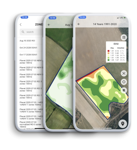
Delineating zones typically uses data-driven factors. Common factors include soil maps and properties (e.g. texture, organic carbon, pH), topography (slope, elevation), historical yield data, and climate or moisture patterns. For example, zones have been delineated using maps of soil organic carbon, electrical conductivity (EC) (which correlates with texture and salinity), sand/silt/clay percentages, and remote-sensing indices like NDVI (Normalized Difference Vegetation Index). In practice, farmers often use whatever data is readily available: aerial or satellite imagery (showing differences in crop growth), yield monitor maps, handheld or vehicle-mounted EC sensors, and traditional soil surveys (e.g. USDA Web Soil Survey). Figuring out zones may involve overlaying these layers or using machine learning methods (clustering the data) to define homogenous areas.

Zone-based management has important advantages over treating a field uniformly. With whole-field (uniform) management, inputs are spread evenly, which means some areas get too much fertilizer (wasteful and polluting) and some too little (lost yield). By contrast, zone management can “optimize the utilization of the input” and “decrease the overall use of chemicals, seed, water, and other inputs”. In other words, feeding the right fertilizer rate to zones that need it, while not wasting it on already rich spots, improves fertilizer-use efficiency and cuts costs.

Studies confirm these benefits: an industry analysis reported that precision technologies (which include zone-based approaches) can increase crop productivity by about 5% while cutting fertilizer use by ~8%, herbicide use by ~9%, water by ~5%, and fuel by ~7%. Zone management also helps protect water quality and soil health by reducing nutrient runoff – for example, careful soil sampling and variable-rate fertilization reduce nitrate leaching into groundwater.

Overall, management zones turn complex in-field variability into actionable units. Well-defined zones should show similar behavior over time (they “have the same yield trend across years”) and respond similarly to inputs. By contrast, uniform management ignores the “real story” of field variation. Zones allow farmers to create prescription maps (variable-rate plans) that match each zone’s potential, boosting yield and profit while minimizing environmental impact.

Principles of Precision Soil Sampling

Precision soil sampling differs from traditional sampling in that it deliberately samples the field at a finer spatial resolution to capture variability. Traditional sampling often means one composite sample per large area of a field (e.g. 1 sample per 20–40 acres), which yields an “averaged representation” of the soil and tends to hide local differences. In contrast, precision sampling breaks the field into many smaller units.

One common method is grid sampling: the field is overlaid with a regular grid of squares (often 1–5 acres each), and each grid cell is sampled and analyzed separately. Smaller grid cells yield more detail but also require more samples and higher cost. For example, a Georgia study found that using 1-acre grid cells captured >80% of field variability in most cases, whereas 5- or 10-acre grids missed much of the variation.

Key principles include sampling density and representativeness. A denser grid (closer sample spacing) can pick up smaller patches of soil difference, improving the accuracy of maps and fertilizer prescriptions. However, each additional sample adds cost in labor and lab analysis, so there is a trade-off. Extension guides often recommend composite samples of 8–15 soil cores per sample to be representative.

For example, Clemson Extension suggests collecting about 8–10 cores per grid sample or 10–15 per management-zone sample. This pooling of many cores per sample helps smooth out small-scale noise and better represents each unit. Sampling teams should also ensure that each sample is collected consistently (same probe depth, consistent mixing) to maintain reliability.

Spatial scale matters. On a small field (a few acres) you might sample densely (e.g. 0.5–1 acre grids), whereas on a very large field you might start with coarser grids or zones. Ultimately the field’s inherent variability should guide the density: very uniform fields need fewer samples, but highly variable fields (patchy soils, old fence lines, drainage changes) justify intensive sampling. Geostatistical tools can help quantify this: if the variogram of a soil property shows a long range of spatial correlation, fewer samples may suffice; if it decays rapidly, more samples are needed. In practice, many growers rely on rules of thumb (e.g. 1-acre or 2.5-acre grids) and then refine sampling once they see the results.

Economics is a crucial consideration. Precision sampling can pay off by reducing fertilizer and lime costs, but the upfront cost of many soil tests can be a hurdle. For example, the Georgia study found that although a 1-acre grid required more samples, it often reduced overall costs by improving fertilizer accuracy. They showed that total input costs (including sampling) were actually lower for the 1-acre grids than for coarser grids, because coarse grids led to heavy under- or over-application of nutrients. Nonetheless, many farmers initially choose larger grids (5–10 acres) simply to lower sampling bills, which risks cutting accuracy. In optimizing design, one should aim for the “sweet spot” – enough samples to capture variability, but no more than needed.

Soil Sampling Strategies for Management Zone Delineation

Agricultural fields are not uniform; soil properties such as nutrient levels, texture, organic matter, and moisture vary from one location to another. Soil sampling helps collect accurate and location-specific soil data, which is essential for defining these zones correctly. Instead of applying the same treatment across the entire field, zone-based soil sampling allows site-specific management, improving input use efficiency, reducing costs, and supporting sustainable farming practices.

4.1 Grid Sampling

Grid sampling is systematic: the field is divided into a uniform grid of cells (square or rectangular). Samples are taken in each cell (often at the center point, called point sampling, or in a zigzag pattern across the cell, called cell sampling). In point sampling, one core or small area is sampled (e.g. center of each cell) and composited in a bucket for that cell. In cell sampling, multiple cores are taken within the cell (often in a zigzag) and then mixed, aiming to represent the whole cell. Point sampling is more labor-intensive (more locations) but captures variability better, whereas cell sampling uses fewer cores but may miss some heterogeneity.

Grid sampling’s advantages include simplicity and uniform coverage with no prior data needed. It is easy to implement with GPS guidance. The main limitation is cost: small grids (e.g. 1 acre) require many samples, while larger grids (e.g. 5–10 acres) may oversimplify the field. The Georgia research found that 1-acre grids achieved ≥80% application accuracy for most nutrients in nearly all fields tested, but 5-acre grids worked poorly except in very uniform fields. In general, finer grids improve accuracy but increase sample count.

A common recommendation is a grid size of ≤2.5 acres for fields with unknown variability. U.S. consultants sometimes use 5-acre grids to save money, but studies suggest this often yields inaccurate soil maps. Ultimately, farmers must balance the higher cost of denser sampling against the benefit of more precise input application (reduced fertilizer waste and yield risk).

4.2 Zone Sampling

Zone sampling (also called directed sampling or stratified sampling) uses pre-defined zones that are believed to be internally homogeneous. These zones may be drawn based on soil maps, yield history, aerial photos, EC maps, topography, or other criteria. For example, a farmer might use known soil types or digital elevation to break the field into a few large zones, then take several soil samples (10–15 cores) from each zone. Often one composite sample is analyzed per zone.

Advantages of zone sampling include fewer total samples (zones are large) and the use of expert knowledge or data to guide sampling. It can save labor, especially if good historical data is available. However, its accuracy depends on how well the zones match real variability. Misclassified zones (e.g. lumping a high-P area with a low-P area) will give misleading results.

In practice, researchers find that zone sampling can be effective but often still less detailed than dense grids. Clemson Extension notes that zone-based plans tend to have larger zones with fewer samples and thus are less costly but also generally less precise than fine-grid maps. A rule of thumb is to use zone sampling when there is reliable historical information; if not, start with grid sampling to build that knowledge.

Often, zone sampling and grid sampling are combined: for instance, using a coarse grid to verify if existing zones are valid. Another approach is to take composite samples within zones: sample several cores along a transect in each zone and mix them, which smooths intra-zone variability. Compared with grid sampling, zone sampling usually reduces analysis costs but may sacrifice some precision. Corteva Agriscience notes that zones are “a better choice” than grids when a farmer has a working history of the field, whereas grids are safer in unknown fields.

4.3 Directed (Targeted) Sampling

Directed sampling is similar to zone sampling but emphasizes using specific data layers to target sample locations. For example, one might overlay a yield map and place extra samples in areas of consistently low yield (to see if soil fertility is causing it). Or one might take samples along gradients of soil EC or NDVI imagery. The idea is to “target” areas that drivers of variability suggest are different. Clemson Extension describes directed sampling as drawing zones from historical yield maps, EC maps, or topographic data. For instance, all low-lying areas (drainage zones) might form one zone, while hilltops form another.

Directed sampling often uses yield maps. As crops are harvested, GPS-equipped combines record yields; mapping these over years can show patterns. Low-yield strips may correlate with soil problems (pH, compaction). Incorporating remote sensing imagery (satellite or drone NDVI, color-infrared) also guides sampling.

For example, a wheat field’s NDVI image might highlight patches where crops are consistently stunted; one would sample those patches intensively. Soil EC scanning (with a Veris or similar) is another directed method: EC correlates with texture and salinity, so zones of similar EC can be sampled separately. SDSU notes that yield monitors and aerial images provide spatial maps that growers use to delineate zones.

Directed sampling can greatly reduce sample count when good data exists, but it requires that data. A drawback is that if the guiding data has anomalies (e.g. one dry year’s yield map), the sampling plan may miss true variability. Therefore, use multi-year data if possible, or combine different sources. For example, if both yield and EC maps point to a particular area as unique, that area clearly merits separate sampling.

4.4 Hybrid Approaches

Hybrid strategies combine grid, zone, and sensor methods. One approach is grid+zone: start with a coarse grid, identify patterns, then refine certain areas into zones or finer subgrids. Another is sensor+soil: use continuous data (like an EC survey or handheld pH sensor) to inform where to take lab samples. For instance, an EC map might show 3 distinct ranges; those become three sampling zones, and within each one or two cores are collected per acre. Many consultants now use this hybrid planning via software: layering sensor maps with yield and soil data, then running clustering algorithms.

Hhybrid sampling uses the strengths of each method. Grid ensures no blind spots; zones incorporate prior information to save effort; sensors provide high-resolution previews of soil variation. Modern planning tools allow farmers to set a grid density for unknown areas while directing extra points to known trouble spots (like “dead zones”). Such flexibility is increasingly common in farm software.

Data Sources Supporting Zone Delineation

Layers are often combined in GIS. For example, one may overlay a yield map, an ECa map, and a satellite image, then visually or algorithmically identify zones where all layers agree on distinctiveness. The Clemson guide notes that combining data from multiple years and types helps avoid basing zones on any single anomaly. In essence, the richer the data sources, the more informed the zone delineation will be. Delineating management zones relies on diverse data sources:

Yield Maps: Modern combines record yields and moisture at GPS locations, producing detailed yield maps. These maps reveal which parts of the field consistently underperform. Overlaid with field boundaries, yield maps often show spatial patterns linked to soil or management. Multi-year yield data are especially powerful for zones.

Soil Electrical Conductivity (ECa): On-the-go EC sensors (e.g. Veris machines) measure soil conductivity, which correlates with soil texture, moisture, salinity, and organic matter. Mapping ECa can highlight soil texture changes (sand vs. clay areas) without lab tests. EC maps are quick and relatively inexpensive and are commonly used in zone planning.

Remote Sensing (Satellite/UAV Imagery): Vegetation indices like NDVI from satellites or drones capture plant vigor, indirectly reflecting soil fertility or moisture differences. High-NDVI areas usually indicate healthy, well-fertilized zones. Multi-spectral imagery (including infrared) can reveal stress not visible to the naked eye. Researchers have found that aerial photos and NDVI often align with yield zones.

Digital Elevation Models (DEM): Elevation data (from LIDAR or GPS) provide slope and aspect information. Topography affects water flow and soil depth; low-lying areas may accumulate clay and salts, while hills are sandier and drier. DEM-based layers (slope, wetness index) can be used to define zones or weight sampling density.

Historical Soil Surveys and Maps: Government soil survey maps (e.g. USDA Web Soil Survey) outline general soil types and map units. These are often coarse-scale but serve as a starting point. Farmers can digitize soil type boundaries from these maps; however, such maps may miss smaller patches, so they should be “ground-truthed” with sampling. Historical records of past fertilizer, lime, or manure applications (if available) can also inform zones of differing fertility.

Geostatistical and Spatial Analysis Methods

In practice, analysts often combine these methods. For example, one might krige soil EC data to create a map, then run k-means clustering on the kriged EC and yield map to define zones. The goal is zones that are statistically distinct (different means for key soil nutrients or yield) and spatially contiguous. After collecting data, statistical and spatial analysis techniques help define and verify zones:

1. Spatial Interpolation (Kriging): Kriging is a geostatistical method that creates continuous surface maps from discrete samples. For example, soil test values (pH, P, K) or yield measurements at sample points can be interpolated using ordinary kriging, which weights nearby samples based on a variogram model. Kriging produces smooth maps of predicted soil nutrients or yield potential. Spatial interpolation is used both to visualize variability and to assess how well sample points capture that variability. A well-chosen variogram model (exponential, Gaussian, etc.) will reflect the field’s autocorrelation structure.

2. Variogram Analysis: The variogram quantifies how data similarity decreases with distance. By fitting a variogram model to sample data, one can determine the “range” (beyond which samples are uncorrelated) and “sill” (variance). A nugget effect indicates unexplained micro-scale variation or measurement error. Knowing the variogram helps decide sampling spacing: if the range is small, points must be close. Variogram parameters are also used in kriging to generate prediction error estimates.

3. Cluster Analysis (e.g. k-means, Fuzzy C-means): Clustering algorithms are often used to group data points (soil samples, yield values, satellite pixels) into zones. K-means clustering partitions the data into a chosen number of zones by minimizing variance within each zone. Fuzzy C-means allows points to belong partially to multiple clusters. Other methods like hierarchical clustering or density-based clustering (DBSCAN) can also delineate zones. Research shows clustering methods are widely used for zone delineation. For example, an Italian study used fuzzy clustering on yield and soil data to define two management zones, achieving strong agreement with actual yield patterns. Software tools like Management Zone Analyst use clustering plus manual review to finalize zones.

4. Principal Component Analysis (PCA): PCA reduces the number of variables by combining correlated factors into principal components. This is useful if many soil properties have been measured. For instance, PCA might find that clay content, sand content, and CEC are correlated, so they combine into one factor. Sci­entific reports have used PCA to identify which soil parameters are most important for zoning; e.g. sand, clay, and organic carbon often emerge as key variables. PCA can also be used to reduce input layers before clustering, improving algorithm performance.

5. GIS-based Techniques: Geographic Information Systems (GIS) provide tools to overlay and analyze all spatial data layers. Techniques include weighted overlay (rating areas by combined soil and yield scores), spatial multi-criteria analysis, and simple visual interpretation. Many farm management software platforms now incorporate GIS routines that allow drawing zones interactively. For example, one might use soil maps as masks in GIS to ensure samples cover each soil type, or use raster clustering tools to segment a combined NDVI+topography layer into zones.

Sampling Design Optimization

Optimization is iterative: start with an informed guess (based on existing data and field size), sample, analyze variability, then refine the design to maximize return on investment. Software planners are increasingly offering tools to suggest optimal sample numbers and locations. Choosing the right sampling design involves balancing accuracy and cost. Key considerations include:

1. Optimal Sampling Intensity: How many samples are needed? This depends on field variability and required confidence. In practice, one might start with a baseline plan (e.g. a grid of 1- or 2-acre cells) and adjust if too few or too many samples seem necessary. UGA researchers tested different grid sizes and found 1-acre grids were optimal for most fields. They recommend starting with a 1-acre grid for a new field (or until a baseline map is made) and later moving to 2.5-acre grids or zone sampling as confidence grows.

2. Spatial Autocorrelation Assessment: By analyzing a few initial samples, one can estimate spatial correlation. High autocorrelation (long variogram range) means the field is fairly uniform at short distances, so fewer samples might suffice. Low autocorrelation (short range) means patchiness – more samples needed. Tools like Moran’s I or variograms are used to assess autocorrelation. If pilot data shows strong spatial structure, one can space samples accordingly.

3. Cost-Benefit Analysis: Economic factors guide design. Each sample has a cost (travel+labor+lab fee). On the other hand, misapplication of fertilizer due to under-sampling can cost more than extra sampling. The Georgia study showed that although 1-acre grids cost more to sample, they often reduced overall fertilizing costs because they avoided over-application on 2.5–5 acre grids. When optimizing, consider the value of reduced uncertainty: for high-value crops or expensive nutrients (like P), it may pay to sample densely.

4. Uncertainty Reduction: Sampling more points reduces the statistical uncertainty of soil estimates. Design of Experiments theory (e.g. stratified random vs. systematic) can be applied. One can use geostatistical confidence intervals to estimate the uncertainty of a map and decide if more samples are needed. In practice, extending the grid or adding random samples in anomalous spots can improve reliability.

5. Validation of Zones: After zones are delineated and sampling done, the accuracy of zones should be validated. This may involve split-sample testing (leave some points out of clustering and see if zones still make sense) or comparing zone-based recommendations against a separate high-density soil grid. In the UGA study, zones or grids were validated by comparing how well they matched a reference high-density sampling. If zones predict yields or nutrient status well, they are validated. Otherwise, adjust the design.

Implementation Workflow

The workflow ensures that management zone delineation is data-driven and actionable. Each step builds on the previous, from collecting raw data to producing a final precision-application plan. Clemson Extension highlights that precision sampling leads to management zones and prescription maps, “increasing the accuracy of rate and placement of necessary inputs”. Putting it all together, a typical workflow for management-zone soil sampling is:

1. Field Data Collection: Gather all existing data layers (yield maps, soil surveys, imagery, EC scans). Define field boundaries in GIS. Choose an initial sampling strategy (grid or zones) based on data availability.
2. Site Reconnaissance: Walk the field or examine maps to note obvious zones (soil color changes, tile drainage lines, erosion spots). Adjust plans if necessary.
3. Soil Sampling: Using GPS guidance, collect soil samples according to the plan. For grids or zones, take 8–15 cores per sample and mix them. Label each sample with its location or zone ID. Keep good records of sample locations (GPS points or maps).
4. Laboratory Analysis: Send samples to a soil lab to analyze pH, nutrients (N, P, K), organic matter, etc. Ensure consistent testing protocols across all samples.
5. Data Preprocessing: Import lab results into GIS or analysis software. Join them to the sampling points. Clean the data (flag any outliers or errors). If needed, perform calibration or normalization.
6. Statistical Analysis: Compute summary statistics for each potential zone (mean pH, etc.). Perform spatial interpolation (kriging) to generate continuous maps of each soil variable. Use variograms to assess spatial structure.
7. Zone Delineation: Use clustering algorithms (e.g. k-means) or GIS overlay methods to delineate zones. For example, run a k-means on normalized soil P, K, and texture maps to divide the field into 3–5 zones. Refine the zones by hand if needed to ensure contiguity.
8. Soil Sampling within Zones: If zones are large and you did an initial grid, you may now switch to zone sampling: take composite samples within each zone for final prescription. Or, if already sampled by zone, verify that enough points were taken in each zone.
9. Prescription Map Generation: Translate zone soil test results into management guidelines. For each zone, calculate the recommended fertilizer or lime rate (using crop nutrient guidelines). Create a variable-rate prescription map (e.g. a color-coded map or GPS guidance lines) for field application equipment.
10. Field Implementation: Upload the prescription map to the farm equipment (planter, sprayer or spreader). Apply inputs according to the zone map in the next planting season.
11. Monitor and Adjust: After harvest, compare yields with the zones and evaluate performance. Collect more data (additional soil or yield maps) in subsequent years to refine zones as needed.

Challenges and Limitations

While management-zone sampling has high potential, its success depends on careful execution and realistic expectations. It works best when variability is real and significant, and when farmers have access to the necessary data and tools. Planning must account for these limitations to yield practical benefits. Despite its benefits, precision soil sampling for zones faces challenges:

Field Variability: Soil and crop variability can be highly complex. Some fields may have random hotspots (e.g. old dump sites) or subtle changes that even dense sampling can miss. Temporal variability (seasonal changes, crop rotation) also complicates interpretation. For instance, moisture differences between wet and dry years can make yield maps misleading if taken from just one season. Managing temporal stability (ensuring zones hold true across years) is a known difficulty.

Sampling Errors: Soil sampling is subject to errors: sampling bias (if GPS points are off), heterogeneity within the sample (if cores are not mixed well), and lab analytical error. These errors introduce noise into the data, which can blur zone boundaries. Strict protocols (consistent sampling depth, probe cleaning, sample handling) are needed to minimize these errors.

Cost Constraints: The biggest barrier is often cost, especially for small or resource-limited farms. Precision equipment and dense soil sampling require investment. The AEM study notes that cost is a major obstacle to adoption. Lower-income farms may skip precision steps even if they know the benefits because of tight budgets. Smaller farms (< $350k sales) lag far behind large farms in adopting precision technology.

Data Integration Complexity: Bringing together multiple data sources (yield, EC, satellite, survey maps) is technically challenging. It requires GIS skills and understanding of different data resolutions and quality. Moreover, these layers may not align perfectly (e.g., old soil maps vs. new satellite images). Farmers often lack the expertise to integrate everything themselves, relying instead on consultants or software tools.

Change in Field Conditions: Fields evolve over time (erosion, management changes, new drainage). Zones defined once may become obsolete. A zone map from five years ago might not reflect current conditions, especially if management has been non-uniform. Continuous monitoring and updating are therefore needed, which adds work.

Adoption Barriers: Beyond cost, there are human barriers. Many farmers are comfortable with traditional methods and skeptical of complex analytics. They may question whether the added complexity of zones is worth it. Effective extension and demonstration are needed to show clear benefits.

Economic and Environmental Implications

Precise soil sampling and zone management can deliver strong economic and environmental gains. By matching fertilizer rates to actual needs, farmers use inputs more efficiently. The AEM/Kearney study quantified this: precision ag can boost overall field productivity by ~5% and reduce key inputs by 5–9%. For example, using site-specific N and P rates rather than flat rates saved an average of 8% fertilizer and 9% herbicide. These savings translate directly into cost reductions for the farmer.

From an environmental standpoint, lower input use means less runoff and leaching. Precision lime and fertilizer application, guided by dense soil maps, minimizes excess nutrient in vulnerable areas. Clemson Extension emphasizes that precision sampling leads to higher nutrient use efficiency and reduced nutrient loss to the environment. This is critical for protecting water quality: when P or N is only applied where needed, there is less chance of it washing into streams or groundwater.

Yield optimization also has broader benefits. Growing more food on the same land reduces the pressure to clear new land, which conserves habitat. If a farmer can get 5% more yield on 1,000 acres, that is 50 extra acres of production-worth of food (and roughly $66,000 more revenue per 1,000 acres for corn, as one analysis estimated). In fact, increased productivity is often cited as the biggest long-term benefit of precision technology: more crops produced using the same (or less) land and resources.

Finally, precision sampling can reduce greenhouse gas emissions. Lower fertilizer rates mean less nitrous oxide emissions from soils, and more efficient equipment use (due to better planning) means less fuel burnt. All of these add up to making farming more sustainable.

Although precision sampling has upfront costs, its economic returns (through saved inputs and higher yields) and environmental payoffs (through reduced pollution and land use) can be substantial. As one review concludes, deploying precision methods “enhances the efficiency of nutrients supplied with fertilizers, as a premise for improved crop yield”.

Case Studies and Applications

Several cases illustrate common findings: zone-based sampling (guided by data) can match the performance of dense grids while using far fewer samples, especially if the chosen data layers truly reflect the underlying variability. Performance is usually measured by metrics like the percent of field areas within 10% of target fertilizer rates, or by comparing zone-defined application maps to high-density “truth” maps. In all cases, careful design and local calibration were key to success. Many real-world examples demonstrate the value of management-zone sampling:

1. University of Georgia Study (2024): Nine cotton and peanut fields in Georgia were sampled at grid sizes from 1 to 10 acres. The researchers found that 1-acre grids achieved ≥80% accuracy in nutrient application in 8 of 9 fields, while 5- and 10-acre grids performed poorly (often ~50% accuracy). Economically, although 1-acre grids involved more lab tests, they actually lowered overall fertilizer costs by avoiding over-application. The study concluded that 1-acre grids were most cost-effective and should be used initially, moving to zone or 2.5-acre grids once the field’s patterns are understood.

2. Brazilian Soybean Fields (Maltauro et al., cited in): In three commercial fields, researchers applied multiple clustering methods (K-means, Fuzzy C-means, etc.) on soil data to define zones. They found two zones each year, and crucially, this zoning allowed farmers to reduce soil samples by 50–75% compared to a uniform grid without losing information. In practice, this means much lower sampling cost with little loss of accuracy in mapping soil fertility.

3. Italian Multi-Year Yield Study (Abid et al., 2022): In a 9-hectare field with 7 years of multi-crop yield data, combined with NDVI satellite imagery and soil analysis, researchers used geostatistics and clustering to delineate zones. They created a two-zone map based on the most correlated soil and NDVI parameters, which agreed with the yield pattern 83% of the time. This confirmed that well-selected zones can represent the field’s productivity pattern.

4. Extension Demonstrations: Various cooperative extension programs have shown that zone sampling can be practical on farm scale. For instance, Clemson’s guide outlines a trial where soil EC mapping and yield maps led to a zone sampling plan in cotton fields. Similarly, Ohio State has documented growers who switched to zone sampling and successfully cut fertilizer use while maintaining yields.

Future Perspectives

The trend is toward more integrated, automated, and data-rich zone delineation. The combination of machine learning, networked sensors, and robotics will likely make precision soil sampling faster and cheaper. Farmers will have tools that can quickly interpret their field’s history and geometry to generate an optimal sampling map. Big data analytics might even predict zones with fewer physical samples by analyzing vast datasets. In all, the future points to precision sampling becoming a routine part of sustainable agriculture. The field of precision soil sampling and zone delineation is rapidly evolving with new technologies:

Machine Learning and AI: Modern software increasingly uses advanced algorithms to create zones. Many platforms now apply ML clustering (e.g. K-means on combined datasets) or even neural-network approaches to optimize zones. These tools can handle large datasets (satellite images, multi-year yields) and generate zones with minimal human bias. For example, some companies allow importing any number of layers (soil, yield, NDVI, DEM) and then automatically compute zones that best capture variability. Early reports suggest ML-based zoning can capture 15–20% more of the field variance than older methods. In the near future, we expect even more automation: software that continuously learns from new data and refines zone boundaries over time.

Real-Time Soil Sensing: On-the-go sensors and robotics promise to gather soil data faster. There are emerging robotic rovers equipped with soil probes and lab-on-chip analyzers, capable of sampling and testing soil nutrients autonomously in the field. Drones are also being tested for soil analysis; for example, drones with hyperspectral sensors could infer pH or moisture patterns. Advances in sensors (for N, K, organic carbon) are making it feasible to get some soil data without digging. The long-term vision is that fields could be continuously monitored, with zoning updated in real time as conditions change.

Automation and Robotics: Tractors and implements are becoming self-driving. In the future, a robotic tractor might follow a prescription map, stop at each zone to collect and test a sample on the spot, and then apply the correct input before moving on, all without human intervention. Several research projects are already exploring autonomous soil sampling vehicles. Meanwhile, “smart” equipment (like variable-rate spreaders with sensors) is pushing more growers to adopt zoning, because they have the machinery to use it.

Big Data and Decision Support: With the explosion of farm data (cloud-based yield databases, national soil databases, etc.), decision-support systems are emerging. These systems integrate big data (e.g. satellite time series, climate forecasts) to recommend zones and application rates. For instance, an online tool might allow a farmer to upload his last 5 years of yield maps and receive back an optimized zone map and soil sampling plan. Data sharing and AI-driven analysis will make sophisticated zone delineation accessible to more growers.

Economic Tools and Policies: As evidence of precision benefits accumulates, we may see more incentives or cost-sharing for zoning. Governments concerned about water quality are interested in these practices. Decision-support programs might include profit calculators: for example, the AEM study’s figures (5% yield gain, etc.) help make the case to farmers and policymakers. In the coming decade, precision sampling plans are likely to become standard practice, much like soil pH testing is today.

Conclusion

Developing effective management zones starts with good soil sampling design. In each case, the goal is to capture the most important soil variability with as few samples as necessary. Successful zone delineation relies on understanding field factors and using appropriate spatial analysis tools to turn that understanding into maps. The central strategy is to tailor the sampling approach to the field. Research and case studies consistently show that precise zone mapping can significantly improve fertilizer efficiency and yield. As the technology landscape evolves, precision soil sampling will only get easier and more powerful. By mapping soil variability accurately, farmers can apply the right input at the right place and time, maximizing productivity and sustainability.